
Don't know much about Bitcoin or price volatility but want to make investment decisions to make a profit? This machine learning model has your back. It can predict prices better than an astrologer. In this article, we will build an ML model for predicting and predicting the price of Bitcoin, using ZenML and MLflow. So let's begin our journey to understand how anyone can use ML and MLOps tools to predict the future.
Learning Objectives
- Learn how to download live data using the API properly.
- Understand what ZenML is, why we use MLflow, and how you can integrate with ZenML.
- Explore the implementation process of machine learning models, from idea to production.
- Discover how to create an easy-to-use Streamlit application for predicting an interactive learning model.
This article was published as part of the Data Science Blogathon.
Problem Statement
Bitcoin prices are very volatile, and making predictions is next to impossible. In our project, we use MLOps best practices to build an LSTM model to predict Bitcoin prices and trends.
Before creating the project, let's look at the project architecture.
Project Implementation
Let's start by accessing the API.
Why do we do this? You can get historical Bitcoin price data from different datasets, but through API, we can access live market data.
Step 1: API access
import requests
import pandas as pd
from dotenv import load_dotenv
import os

# Load the .env file
load_dotenv()

def fetch_crypto_data(api_uri):
    response = requests.get(
        api_uri,
        params={
            "market": "cadli",
            "instrument": "BTC-USD",
            "limit": 5000,
            "aggregate": 1,
            "fill": "true",
            "apply_mapping": "true",
            "response_format": "JSON"
        },
        headers={"Content-type": "application/json; charset=UTF-8"}
    )

    if response.status_code == 200:
        print('API Connection Successful! nFetching the data...')

        data = response.json()
        data_list = data.get('Data', [])

        df = pd.DataFrame(data_list)

        df['DATE'] = pd.to_datetime(df['TIMESTAMP'], unit="s")

        return df  # Return the DataFrame
    else:
        raise Exception(f"API Error: {response.status_code} - {response.text}")
Step 2: Connecting to the database using MongoDB
MongoDB is a NoSQL database known for its flexibility, extensibility, and ability to store unstructured data in a JSON-like format.
import os
from pymongo import MongoClient
from dotenv import load_dotenv
from data.management.api import fetch_crypto_data  # Import the API function
import pandas as pd

load_dotenv()

MONGO_URI = os.getenv("MONGO_URI")
API_URI = os.getenv("API_URI")

client = MongoClient(MONGO_URI, ssl=True, ssl_certfile=None, ssl_ca_certs=None)
db = client['crypto_data']
collection = db['historical_data']

try:
    latest_entry = collection.find_one(sort=[("DATE", -1)])  # Find the latest date
    if latest_entry:
        last_date = pd.to_datetime(latest_entry['DATE']).strftime('%Y-%m-%d')
    else:
        last_date="2011-03-27"  # Default start date if MongoDB is empty

    print(f"Fetching data starting from {last_date}...")
    new_data_df = fetch_crypto_data(API_URI)

    if latest_entry:
        new_data_df = new_data_df[new_data_df['DATE'] > last_date]

    if not new_data_df.empty:
        data_to_insert = new_data_df.to_dict(orient="records")
        result = collection.insert_many(data_to_insert)
        print(f"Inserted {len(result.inserted_ids)} new records into MongoDB.")
    else:
        print("No new data to insert.")
except Exception as e:
    print(f"An error occurred: {e}")
This code connects to MongoDB, retrieves Bitcoin price data via the API, and updates the database with all new entries after the latest entry date.
Introducing ZenML
ZenML is an open source platform designed for machine learning, supporting the creation of flexible and production-ready pipelines. In addition, ZenML also includes many machine learning tools such as MLflow, BentoML, etc., to create seamless ML pipelines.
⚠️ If you are a Windows user, try installing wsl on your system. Zenml does not support Windows.
In this project, we will use a common pipeline, which uses ZenML, and we will be integrating MLflow with ZenML, to track the tests.
Prerequisites and instructions for Basic ZenML
#create a virtual environment
python3 -m venv venv

#Activate your virtual environmnent in your project folder
source venv/bin/activate- ZenML commands:
All core ZenML commands and their functionality are given below:
#Install zenml
pip install zenml

#To Launch zenml server and dashboard locally
pip install "zenml[server]"

#To check the zenml Version:
zenml version

#To initiate a new repository
zenml init

#To run the dashboard locally:
zenml login --local

#To know the status of our zenml Pipelines
zenml show

#To shutdown the zenml server
zenml clean
Step 3: Integration of MLflow and ZenML
We use MLflow to track tests, track our model, artifacts, metrics, and hyperparameter values. We list the MLflow test tracker and model builder here:
#Integrating mlflow with ZenML
zenml integration install mlflow -y
#Register the experiment tracker
zenml experiment-tracker register mlflow_tracker --flavor=mlflow
#Registering the model deployer
zenml model-deployer register mlflow --flavor=mlflow
#Registering the stack
zenml stack register local-mlflow-stack-new -a default -o default -d mlflow -e mlflow_tracker --set
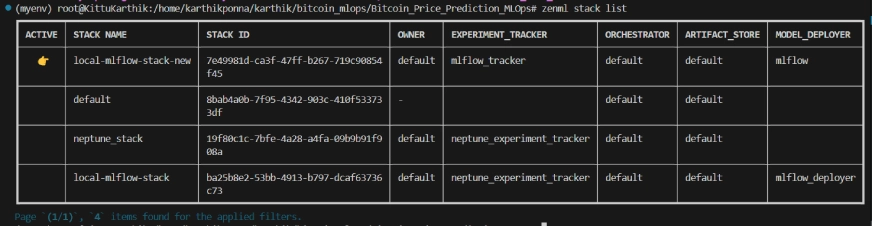
#To view the stack list
zenml stack --listZenML Stack List
Project Structure
Here, you can see the project structure. Now let's discuss them one by one in detail.
bitcoin_price_prediction_mlops/        # Project directory
├── data/
│   └── management/
│       ├── api_to_mongodb.py          # Code to fetch data and save it to MongoDB
│       └── api.py                     # API-related utility functions
│
├── pipelines/
│   ├── deployment_pipeline.py         # Deployment pipeline
│   └── training_pipeline.py           # Training pipeline
│
├── saved_models/                      # Directory for storing trained models
├── saved_scalers/                     # Directory for storing scalers used in data preprocessing
│
├── src/                               # Source code
│   ├── data_cleaning.py               # Data cleaning and preprocessing
│   ├── data_ingestion.py              # Data ingestion
│   ├── data_splitter.py               # Data splitting
│   ├── feature_engineering.py         # Feature engineering
│   ├── model_evaluation.py            # Model evaluation
│   └── model_training.py              # Model training
│
├── steps/                             # ZenML steps
│   ├── clean_data.py                  # ZenML step for cleaning data
│   ├── data_splitter.py               # ZenML step for data splitting
│   ├── dynamic_importer.py            # ZenML step for importing dynamic data
│   ├── feature_engineering.py         # ZenML step for feature engineering
│   ├── ingest_data.py                 # ZenML step for data ingestion
│   ├── model_evaluation.py            # ZenML step for model evaluation
│   ├── model_training.py              # ZenML step for training the model
│   ├── prediction_service_loader.py   # ZenML step for loading prediction services
│   ├── predictor.py                   # ZenML step for prediction
│   └── utils.py                       # Utility functions for steps
│
├── .env                               # Environment variables file
├── .gitignore                         # Git ignore file
│
├── app.py                             # Streamlit user interface app
│
├── README.md                          # Project documentation
├── requirements.txt                   # List of required packages
├── run_deployment.py                  # Code for running deployment and prediction pipeline
├── run_pipeline.py                    # Code for running training pipeline
└── .zen/                              # ZenML directory (created automatically after ZenML initialization)
Step 4: Data Entry
We start by importing data from the API to MongoDB and then converting it to a pandas DataFrame.
import os
import logging
from pymongo import MongoClient
from dotenv import load_dotenv
from zenml import step
import pandas as pd

# Load the .env file
load_dotenv()

# Get MongoDB URI from environment variables
MONGO_URI = os.getenv("MONGO_URI")

def fetch_data_from_mongodb(collection_name:str, database_name:str):
    """
    Fetches data from MongoDB and converts it into a pandas DataFrame.

    collection_name:
        Name of the MongoDB collection to fetch data.
    database_name:
        Name of the MongoDB database.
    return:
        A pandas DataFrame containing the data
    """
    # Connect to the MongoDB client
    client = MongoClient(MONGO_URI)
    db = client[database_name]  # Select the database
    collection = db[collection_name]  # Select the collection

    # Fetch all documents from the collection
    try:
        logging.info(f"Fetching data from MongoDB collection: {collection_name}...")
        data = list(collection.find())  # Convert cursor to a list of dictionaries

        if not data:
            logging.info("No data found in the MongoDB collection.")


        # Convert the list of dictionaries into a pandas DataFrame
        df = pd.DataFrame(data)

        # Drop the MongoDB ObjectId field if it exists (optional)
        if '_id' in df.columns:
            df = df.drop(columns=['_id'])

        logging.info("Data successfully fetched and converted to a DataFrame!")
        return df

    except Exception as e:
        logging.error(f"An error occurred while fetching data: {e}")
        raise e


@step(enable_cache=False)
def ingest_data(collection_name: str = "historical_data", database_name: str = "crypto_data") -> pd.DataFrame:

    logging.info("Started data ingestion process from MongoDB.")

    try:
        # Use the fetch_data_from_mongodb function to fetch data
        df = fetch_data_from_mongodb(collection_name=collection_name, database_name=database_name)

        if df.empty:
            logging.warning("No data was loaded. Check the collection name or the database content.")
        else:
            logging.info(f"Data ingestion completed. Number of records loaded: {len(df)}.")

        return df

    except Exception as e:
        logging.error(f"Error while reading data from {collection_name} in {database_name}: {e}")
        raise e
we add @step as a decorator in import_data() job posting as a step in our training pipeline. In the same way, we will write the code for each step in the construction of the project and create a pipeline.
To see how I used the @step decorator, check out the GitHub link below (steps folder) to walk through the code for other steps in the pipeline i.e. data cleaning, feature engineering, data segmentation, model training, and model testing.
Step 5: Data cleaning
In this step, we will create different techniques to clean the imported data. We will discard unwanted columns and missing values from the data.
class DataPreprocessor:
    def __init__(self, data: pd.DataFrame):

        self.data = data
        logging.info("DataPreprocessor initialized with data of shape: %s", data.shape)

    def clean_data(self) -> pd.DataFrame:
        """
        Performs data cleaning by removing unnecessary columns, dropping columns with missing values,
        and returning the cleaned DataFrame.

        Returns:
            pd.DataFrame: The cleaned DataFrame with unnecessary and missing-value columns removed.
        """
        logging.info("Starting data cleaning process.")

        # Drop unnecessary columns, including '_id' if it exists
        columns_to_drop = [
            'UNIT', 'TYPE', 'MARKET', 'INSTRUMENT',
            'FIRST_MESSAGE_TIMESTAMP', 'LAST_MESSAGE_TIMESTAMP',
            'FIRST_MESSAGE_VALUE', 'HIGH_MESSAGE_VALUE', 'HIGH_MESSAGE_TIMESTAMP',
            'LOW_MESSAGE_VALUE', 'LOW_MESSAGE_TIMESTAMP', 'LAST_MESSAGE_VALUE',
            'TOTAL_INDEX_UPDATES', 'VOLUME_TOP_TIER', 'QUOTE_VOLUME_TOP_TIER',
            'VOLUME_DIRECT', 'QUOTE_VOLUME_DIRECT', 'VOLUME_TOP_TIER_DIRECT',
            'QUOTE_VOLUME_TOP_TIER_DIRECT', '_id'  # Adding '_id' to the list
        ]
        logging.info("Dropping columns: %s")
        self.data = self.drop_columns(self.data, columns_to_drop)

        # Drop columns where the number of missing values is greater than 0
        logging.info("Dropping columns with missing values.")
        self.data = self.drop_columns_with_missing_values(self.data)

        logging.info("Data cleaning completed. Data shape after cleaning: %s", self.data.shape)
        return self.data

    def drop_columns(self, data: pd.DataFrame, columns: list) -> pd.DataFrame:
        """
        Drops specified columns from the DataFrame.

        Returns:
            pd.DataFrame: The DataFrame with the specified columns removed.
        """
        logging.info("Dropping columns: %s", columns)
        return data.drop(columns=columns, errors="ignore")

    def drop_columns_with_missing_values(self, data: pd.DataFrame) -> pd.DataFrame:
        """
        Drops columns with any missing values from the DataFrame.

        Parameters:
            data: pd.DataFrame
                The DataFrame from which columns with missing values will be removed.

        Returns:
            pd.DataFrame: The DataFrame with columns containing missing values removed.
        """
        missing_columns = data.columns[data.isnull().sum() > 0]
        if not missing_columns.empty:
            logging.info("Columns with missing values: %s", missing_columns.tolist())
        else:
            logging.info("No columns with missing values found.")
        return data.loc[:, data.isnull().sum() == 0]
Step 6: Feature engineering
This step takes the cleaned data from the previous_data_cleaning step. We developed new features such as Simple Moving Average (SMA), Exponential Moving Average (EMA), and reactive and convolutional statistics to capture trends, reduce noise, and make more reliable predictions from time series data. Additionally, we scale features and target variables using Minmax scaling.
import joblib
import pandas as pd
from abc import ABC, abstractmethod
from sklearn.preprocessing import MinMaxScaler


# Abstract class for Feature Engineering strategy
class FeatureEngineeringStrategy(ABC):
    @abstractmethod
    def generate_features(self, df: pd.DataFrame) -> pd.DataFrame:
        pass


# Concrete class for calculating SMA, EMA, RSI, and other features
class TechnicalIndicators(FeatureEngineeringStrategy):
    def generate_features(self, df: pd.DataFrame) -> pd.DataFrame:

        # Calculate SMA, EMA, and RSI
        df['SMA_20'] = df['CLOSE'].rolling(window=20).mean()
        df['SMA_50'] = df['CLOSE'].rolling(window=50).mean()
        df['EMA_20'] = df['CLOSE'].ewm(span=20, adjust=False).mean()

        # Price difference features
        df['OPEN_CLOSE_diff'] = df['OPEN'] - df['CLOSE']
        df['HIGH_LOW_diff'] = df['HIGH'] - df['LOW']
        df['HIGH_OPEN_diff'] = df['HIGH'] - df['OPEN']
        df['CLOSE_LOW_diff'] = df['CLOSE'] - df['LOW']

        # Lagged features
        df['OPEN_lag1'] = df['OPEN'].shift(1)
        df['CLOSE_lag1'] = df['CLOSE'].shift(1)
        df['HIGH_lag1'] = df['HIGH'].shift(1)
        df['LOW_lag1'] = df['LOW'].shift(1)

        # Rolling statistics
        df['CLOSE_roll_mean_14'] = df['CLOSE'].rolling(window=14).mean()
        df['CLOSE_roll_std_14'] = df['CLOSE'].rolling(window=14).std()

        # Drop rows with missing values (due to rolling windows, shifts)
        df.dropna(inplace=True)

        return df

# Abstract class for Scaling strategy
class ScalingStrategy(ABC):
    @abstractmethod
    def scale(self, df: pd.DataFrame, features: list, target: str):
        pass

# Concrete class for MinMax Scaling
class MinMaxScaling(ScalingStrategy):
    def scale(self, df: pd.DataFrame, features: list, target: str):
        """
        Scales the features and target using MinMaxScaler.

        Parameters:
            df: pd.DataFrame
                The DataFrame containing the features and target.
            features: list
                List of feature column names.
            target: str
                The target column name.

        Returns:
            pd.DataFrame, pd.DataFrame: Scaled features and target
        """
        scaler_X = MinMaxScaler(feature_range=(0, 1))
        scaler_y = MinMaxScaler(feature_range=(0, 1))

        X_scaled = scaler_X.fit_transform(df[features].values)
        y_scaled = scaler_y.fit_transform(df[[target]].values)

        joblib.dump(scaler_X, 'saved_scalers/scaler_X.pkl')
        joblib.dump(scaler_y, 'saved_scalers/scaler_y.pkl')

        return X_scaled, y_scaled, scaler_y


# FeatureEngineeringContext: This will use the Strategy Pattern
class FeatureEngineering:
    def __init__(self, feature_strategy: FeatureEngineeringStrategy, scaling_strategy: ScalingStrategy):
        self.feature_strategy = feature_strategy
        self.scaling_strategy = scaling_strategy

    def process_features(self, df: pd.DataFrame, features: list, target: str):
        # Generate features using the provided strategy
        df_with_features = self.feature_strategy.generate_features(df)

        # Scale features and target using the provided strategy
        X_scaled, y_scaled, scaler_y = self.scaling_strategy.scale(df_with_features, features, target)

        return df_with_features, X_scaled, y_scaled, scaler_y
Step 7: Data Classification
Now, we divide the processed data into training and testing datasets with a ratio of 80:20.
import logging
from abc import ABC, abstractmethod
import numpy as np
from sklearn.model_selection import train_test_split

# Set up logging configuration
logging.basicConfig(level=logging.INFO, format="%(asctime)s - %(levelname)s - %(message)s")

# Abstract Base Class for Data Splitting Strategy
class DataSplittingStrategy(ABC):
    @abstractmethod
    def split_data(self, X: np.ndarray, y: np.ndarray):
        pass

# Concrete Strategy for Simple Train-Test Split
class SimpleTrainTestSplitStrategy(DataSplittingStrategy):
    def __init__(self, test_size=0.2, random_state=42):

        self.test_size = test_size
        self.random_state = random_state

    def split_data(self, X: np.ndarray, y: np.ndarray):

        logging.info("Performing simple train-test split.")
        X_train, X_test, y_train, y_test = train_test_split(
            X, y, test_size=self.test_size, random_state=self.random_state
        )
        logging.info("Train-test split completed.")
        return X_train, X_test, y_train, y_test

# Context Class for Data Splitting
class DataSplitter:
    def __init__(self, strategy: DataSplittingStrategy):

        self._strategy = strategy

    def set_strategy(self, strategy: DataSplittingStrategy):

        logging.info("Switching data splitting strategy.")
        self._strategy = strategy

    def split(self, X: np.ndarray, y: np.ndarray):

        logging.info("Splitting data using the selected strategy.")
        return self._strategy.split_data(X, y)
Step 8: Model Training
In this step, we train the LSTM model by stopping early to prevent overfitting, and by using MLflow's automatic logging to track our model and test and save the trained model as lstm_model.keras.
import numpy as np
import logging
import mlflow
from tensorflow.keras.models import Sequential
from tensorflow.keras.layers import Input, LSTM, Dropout, Dense
from tensorflow.keras.regularizers import l2
from tensorflow.keras.callbacks import EarlyStopping
from typing import Any
# Abstract Base Class for Model Building Strategy
class ModelBuildingStrategy:
def build_and_train_model(self, X_train: np.ndarray, y_train: np.ndarray, fine_tuning: bool = False) -> Any:
pass
# Concrete Strategy for LSTM Model
class LSTMModelStrategy(ModelBuildingStrategy):
def build_and_train_model(self, X_train: np.ndarray, y_train: np.ndarray, fine_tuning: bool = False) -> Any:
"""
Trains an LSTM model on the provided training data.
Parameters:
X_train (np.ndarray): The training data features.
y_train (np.ndarray): The training data labels/target.
fine_tuning (bool): Not applicable for LSTM, defaults to False.
Returns:
tf.keras.Model: A trained LSTM model.
"""
logging.info("Building and training the LSTM model.")
# MLflow autologging
mlflow.tensorflow.autolog()
logging.info(f"shape of X_train:{X_train.shape}")
# LSTM Model Definition
model = Sequential()
model.add(Input(shape=(X_train.shape[1], X_train.shape[2])))
model.add(LSTM(units=50, return_sequences=True, kernel_regularizer=l2(0.01)))
model.add(Dropout(0.3))
model.add(LSTM(units=50, return_sequences=False))
model.add(Dropout(0.2))
model.add(Dense(units=1)) # Adjust the number of units based on your output (e.g., regression or classification)
# Compiling the model
model.compile(optimizer="adam", loss="mean_squared_error")
# Early stopping to avoid overfitting
early_stopping = EarlyStopping(monitor="val_loss", patience=10, restore_best_weights=True)
# Fit the model
history = model.fit(
X_train,
y_train,
epochs=50,
batch_size=32,
validation_split=0.1,
callbacks=[early_stopping],
verbose=1
)
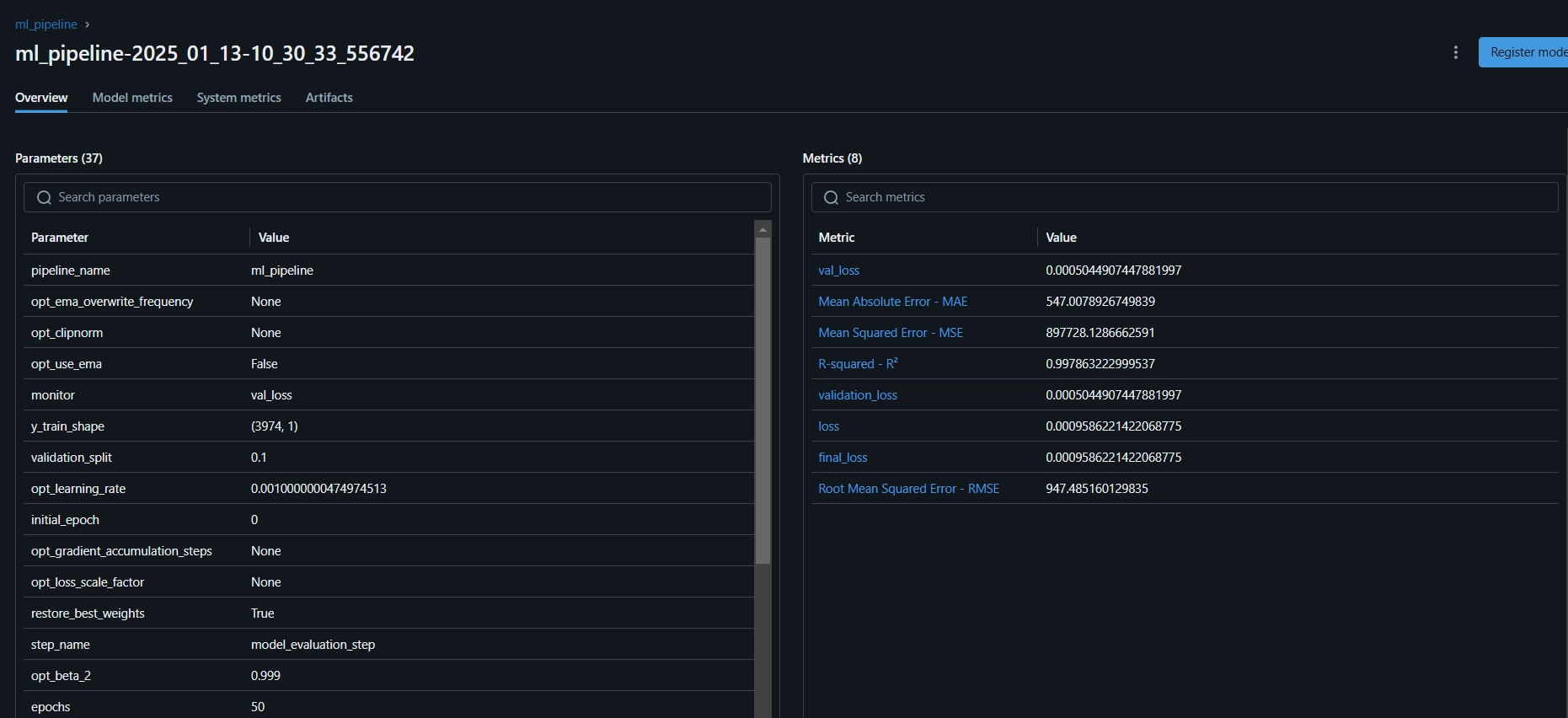
mlflow.log_metric("final_loss", history.history["loss"][-1])
# Saving the trained model
model.save("saved_models/lstm_model.keras")
logging.info("LSTM model trained and saved.")
return model
# Context Class for Model Building Strategy
class ModelBuilder:
def __init__(self, strategy: ModelBuildingStrategy):
self._strategy = strategy
def set_strategy(self, strategy: ModelBuildingStrategy):
self._strategy = strategy
def train(self, X_train: np.ndarray, y_train: np.ndarray, fine_tuning: bool = False) -> Any:
return self._strategy.build_and_train_model(X_train, y_train, fine_tuning)Step 9: Testing the Model
Since this is a regression problem, we use test metrics such as Mean Squared Error (MSE), Root Mean Squared Error (MSE), Mean Absolute Error (MAE), and R-squared.
import logging
import numpy as np
from abc import ABC, abstractmethod
from sklearn.preprocessing import MinMaxScaler
from sklearn.metrics import mean_squared_error, mean_absolute_error, r2_score
from typing import Dict

# Setup logging configuration
logging.basicConfig(level=logging.INFO, format="%(asctime)s - %(levelname)s - %(message)s")

# Abstract Base Class for Model Evaluation Strategy
class ModelEvaluationStrategy(ABC):
    @abstractmethod
    def evaluate_model(self, model, X_test, y_test, scaler_y) -> Dict[str, float]:
        pass

# Concrete Strategy for Regression Model Evaluation
class RegressionModelEvaluationStrategy(ModelEvaluationStrategy):
    def evaluate_model(self, model, X_test, y_test, scaler_y) -> Dict[str, float]:
        # Predict the data
        y_pred = model.predict(X_test)

        # Ensure y_test and y_pred are reshaped into 2D arrays for inverse transformation
        y_test_reshaped = y_test.reshape(-1, 1)
        y_pred_reshaped = y_pred.reshape(-1, 1)

        # Inverse transform the scaled predictions and true values
        y_pred_rescaled = scaler_y.inverse_transform(y_pred_reshaped)
        y_test_rescaled = scaler_y.inverse_transform(y_test_reshaped)

        # Flatten the arrays to ensure they are 1D
        y_pred_rescaled = y_pred_rescaled.flatten()
        y_test_rescaled = y_test_rescaled.flatten()

        # Calculate evaluation metrics
        mse = mean_squared_error(y_test_rescaled, y_pred_rescaled)
        rmse = np.sqrt(mse)
        mae = mean_absolute_error(y_test_rescaled, y_pred_rescaled)
        r2 = r2_score(y_test_rescaled, y_pred_rescaled)

        # Logging the metrics
        logging.info("Calculating evaluation metrics.")
        metrics = {
            "Mean Squared Error - MSE": mse,
            "Root Mean Squared Error - RMSE": rmse,
            "Mean Absolute Error - MAE": mae,
            "R-squared - R²": r2
        }

        logging.info(f"Model Evaluation Metrics: {metrics}")
        return metrics

# Context Class for Model Evaluation
class ModelEvaluator:
    def __init__(self, strategy: ModelEvaluationStrategy):

        self._strategy = strategy

    def set_strategy(self, strategy: ModelEvaluationStrategy):

        logging.info("Switching model evaluation strategy.")
        self._strategy = strategy

    def evaluate(self, model, X_test, y_test, scaler_y) -> Dict[str, float]:

        logging.info("Evaluating the model using the selected strategy.")
        return self._strategy.evaluate_model(model, X_test, y_test, scaler_y)
Now we will organize all the above steps into a pipeline. Let's create a new file training_pipeline.py.
from zenml import Model, pipeline

@pipeline(
    model=Model(
        # The name uniquely identifies this model
        name="bitcoin_price_predictor"
    ),
)
def ml_pipeline():
    # Data Ingestion Step
    raw_data = ingest_data()
    # Data Cleaning Step
    cleaned_data = clean_data(raw_data)
    # Feature Engineering Step
    transformed_data, X_scaled, y_scaled, scaler_y = feature_engineering_step(
        cleaned_data
    )
    # Data Splitting
    X_train, X_test, y_train, y_test = data_splitter_step(X_scaled=X_scaled, y_scaled=y_scaled)
    # Model Training
    model = model_training_step(X_train, y_train)
    # Model Evaluation
    evaluator = model_evaluation_step(model, X_test=X_test, y_test=y_test, scaler_y= scaler_y)

    return evaluator
Here, @pipeline decorator is used to define the ml_pipeline() function as a pipeline in ZenML.
To view the training pipeline dashboard, simply run the run_pipeline.py script. Let's create a run_pipeline.py file.
import click
from pipelines.training_pipeline import ml_pipeline

@click.command()
def main():
    run = ml_pipeline()

if __name__=="__main__":
    main()
Now we have finished building the pipeline. Run the command below to view the pipelines dashboard.
python run_pipeline.pyAfter running the above command it will return the tracking dashboard URL, which looks like this.
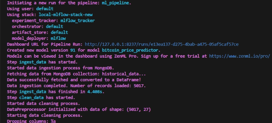
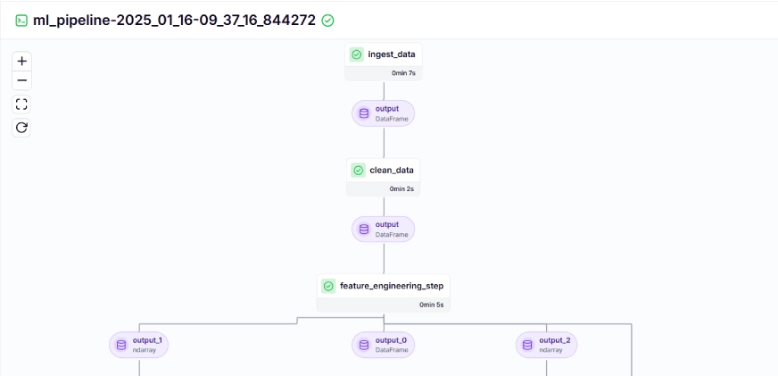
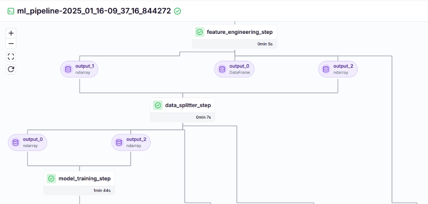
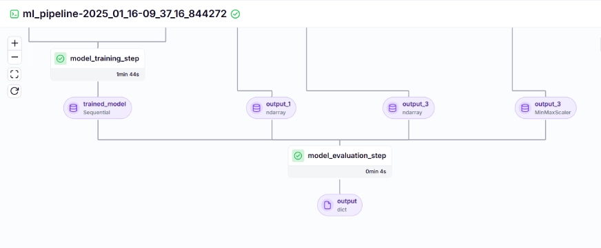
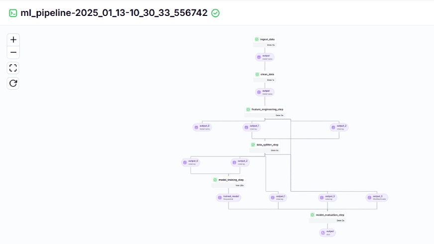
The training pipeline looks like this on the dashboard, given below:
Step 10: Model Deployment
So far we have built the model and pipes. Now let's push the pipeline to production where users can make predictions.
Continuous Delivery Pipeline
from zenml.integrations.mlflow.steps import mlflow_model_deployer_step

@pipeline
def continuous_deployment_pipeline():
    trained_model = ml_pipeline()
    mlflow_model_deployer_step(workers=3,deploy_decision=True,model=trained_model,)
This pipeline is responsible for continuously releasing trained models. It starts running the ml_pipeline() from the train_pipeline.py file to train the model, then use the Mlflow Model Deployer feeding the trained model using the continuous_pipeline().
The Inference Pipeline
We use an inference pipeline to make predictions on new data, using an applied model. Let's see how to use this pipeline in our project.
@pipeline
def inference_pipeline(enable_cache=True):
    """Run a batch inference job with data loaded from an API."""
    batch_data = dynamic_importer()
    model_deployment_service = prediction_service_loader(
        pipeline_name="continuous_deployment_pipeline",
        step_name="mlflow_model_deployer_step",
    )
    predictor(service=model_deployment_service, input_data=batch_data)
Let's see about each of the functions called indexing pipeline below:
dynamic_importer()
This function loads new data, performs data processing, and returns data.
@step
def dynamic_importer() -> str:
    """Dynamically imports data for testing the model with expected columns."""

    try:
        data = {
            'OPEN': [0.98712925, 1.],'HIGH': [0.57191823, 0.55107652],'LOW': [1., 0.94728144],'VOLUME': [0.18186191, 0.],'SMA_20': [0.90819243, 1.],'SMA_50': [0.90214911, 1.],'EMA_20': [0.89735654, 1.],'OPEN_CLOSE_diff': [0.61751032, 0.57706902],'HIGH_LOW_diff': [0.01406254, 0.02980481],
            'HIGH_OPEN_diff': [0.13382262, 0.09172282],
            'CLOSE_LOW_diff': [0.14140073, 0.28523136],'OPEN_lag1': [0.64467168, 1.],
            'CLOSE_lag1': [0.98712925, 1.],
            'HIGH_lag1': [0.77019885, 0.57191823],
            'LOW_lag1': [0.64465093, 1.],
            'CLOSE_roll_mean_14': [0.94042809, 1.],'CLOSE_roll_std_14': [0.22060724, 0.35396897],
        }

        df = pd.DataFrame(data)
        data_array = df.iloc[0].values
        reshaped_data = data_array.reshape((1, 1, data_array.shape[0]))  # Single sample, 1 time step, 17 features

        logging.info(f"Reshaped Data: {reshaped_data.shape}")

        json_data = pd.DataFrame(reshaped_data.reshape((reshaped_data.shape[0], reshaped_data.shape[2]))).to_json(orient="split")

        return json_data

    except Exception as e:
        logging.error(f"Error during importing data from dynamic importer: {e}")
        raise e
predict_service_loader()
This work is decorated with it @step. We load the application service along with the applied model based on pipeline_name, and step_name, when our applied model is ready to process new data prediction queries.
The row where_services=mlflow_model_deployer_component.find_model_server() searches for an available service to use based on the given parameters such as pipe name and pipe step name. If no services are available, it indicates that the deployment pipeline was not created or encountered a problem with the deployment pipeline, so it throws a RuntimeError.
@step(enable_cache=False)
def prediction_service_loader(pipeline_name: str, step_name: str) -> MLFlowDeploymentService:
    model_deployer = MLFlowModelDeployer.get_active_model_deployer()

    existing_services = model_deployer.find_model_server(
        pipeline_name=pipeline_name,
        pipeline_step_name=step_name,
    )

    if not existing_services:
        raise RuntimeError(
            f"No MLflow prediction service deployed by the "
            f"{step_name} step in the {pipeline_name} "
            f"pipeline is currently "
            f"running."
        )
    return existing_services[0]
predict()
The function takes the model supplied by MLFlow via the MLFlowDeploymentService and the new data. The data is continuously processed to match the model's expected format for real-time guidance.
@step(enable_cache=False)
def predictor(
    service: MLFlowDeploymentService,
    input_data: str,
) -> np.ndarray:

    service.start(timeout=10)

    try:
        data = json.loads(input_data)
        data.pop("columns", None)
        data.pop("index", None)

        if isinstance(data["data"], list):
            data_array = np.array(data["data"])
        else:
            raise ValueError("The data format is incorrect, expected a list under 'data'.")

        if data_array.shape != (1, 1, 17):
            data_array = data_array.reshape((1, 1, 17))  # Adjust the shape as needed

        try:
            prediction = service.predict(data_array)
        except Exception as e:
            raise ValueError(f"Prediction failed: {e}")
        return prediction

    except json.JSONDecodeError:
        raise ValueError("Invalid JSON format in the input data.")
    except KeyError as e:
        raise ValueError(f"Missing expected key in input data: {e}")
    except Exception as e:
        raise ValueError(f"An error occurred during data processing: {e}")
To visualize the continuous deployment and targeting pipeline, we need to use the run_deployment.py script, where configuration and prediction will be defined. (Please check the run_deployment.py code on GitHub given below).
@click.option(
    "--config",
    type=click.Choice([DEPLOY, PREDICT, DEPLOY_AND_PREDICT]),
    default=DEPLOY_AND_PREDICT,
    help="Optionally you can choose to only run the deployment "
    "pipeline to train and deploy a model (`deploy`), or to "
    "only run a prediction against the deployed model "
    "(`predict`). By default both will be run "
    "(`deploy_and_predict`).",
)
Now let's use the run_deployment.py file to see the dashboard of the continuous deployment pipeline and the reference pipeline.
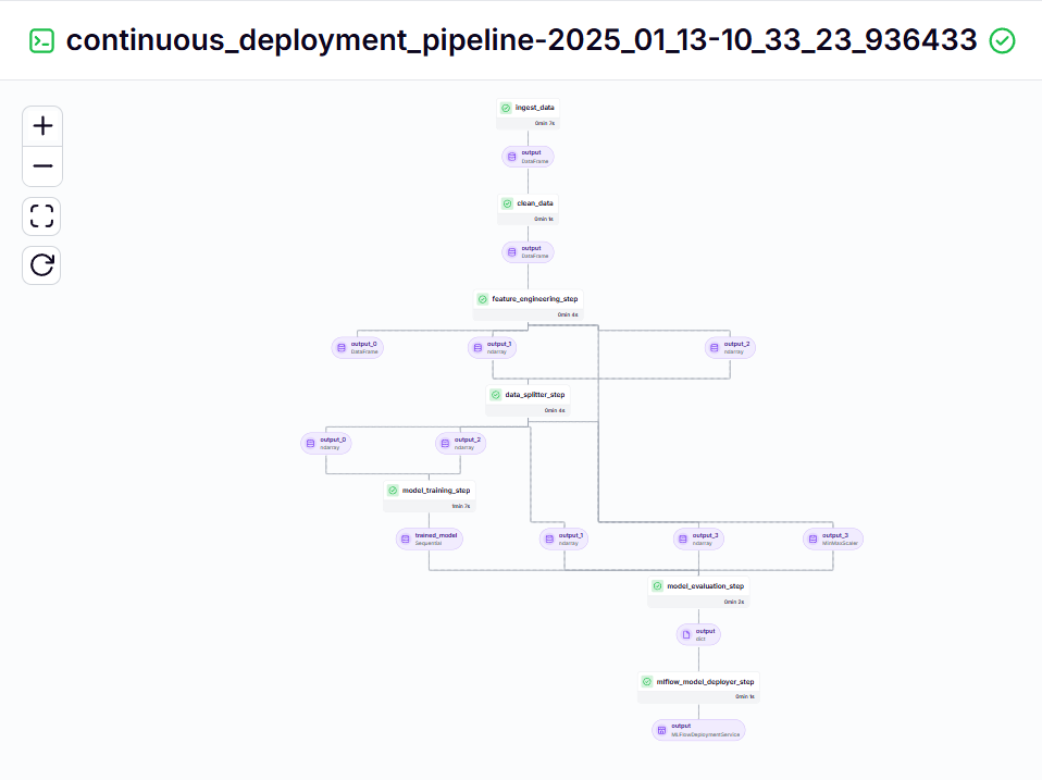
python run_deployment.pyContinuous Delivery Pipeline – Output
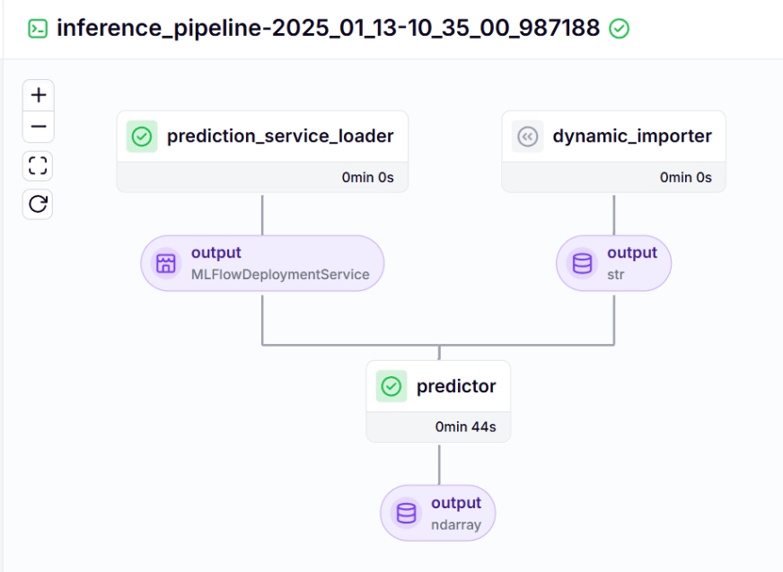
Inference Pipeline – Output
After running the run_deployment.py file you can see a link to the MLflow dashboard that looks like this.
mlflow ui --backend-store-uri file:/root/.config/zenml/local_stores/cd1eb06a-179a-4f83-9bae-9b9a5b1bd27f/mlrunsNow you need to copy and paste the above MLflow UI link into your command line and run it.
Here is the MLflow dashboard, where you can see the test metrics and model parameters:
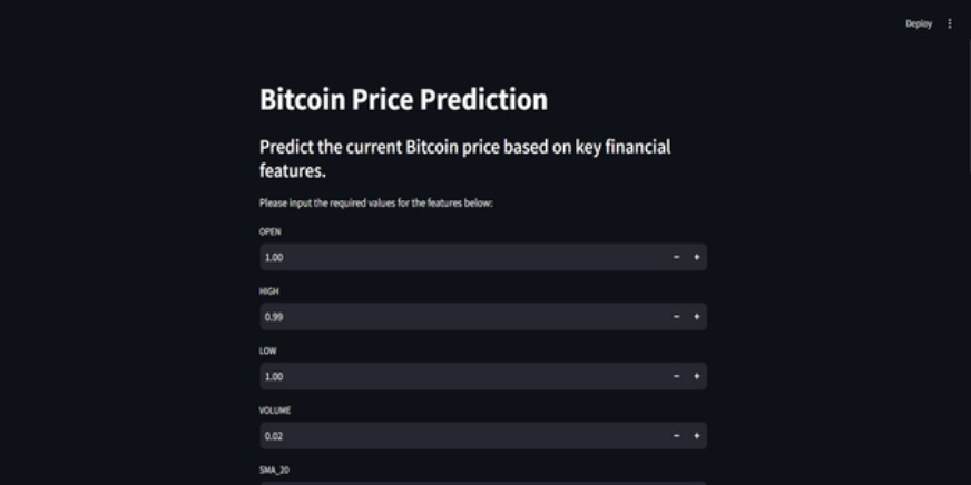
Step 11: Creating a Streaming App
Streamlit is an amazing open source, Python-based framework, used to create interactive UIs, we can use Streamlit to build web applications quickly, without knowing backend or frontend development. First, we need to install Streamlit on our system.
#Install streamlit in our local PC
pip install streamlit

#To run the streamlit local web server
streamlit run app.py
Also, you can find the code on GitHub for the Streamlit app.
Here is GitHub Code and Project Video Description for better understanding.
The conclusion
In this article, we have successfully built an end-to-end, production-ready Bitcoin Price Prediction MLOps project. From getting data through an API and preprocessing it to model training, testing, and deployment, our project highlights the important role of MLOps in connecting development and production. We are close to shaping the future of real-time Bitcoin price prediction. APIs provide seamless access to external data, such as Bitcoin price data from the CCData API, eliminating the need for pre-existing datasets.
Key Takeaways
- APIs enable seamless access to external data, such as Bitcoin price data from the CCata API, eliminating the need for existing datasets.
- ZenML and MLflow are powerful tools that facilitate the development, tracking, and implementation of machine learning models in real-world applications.
- We followed best practices for optimizing data import, cleaning, feature engineering, model training, and testing.
- Continuous distribution and targeting pipelines are essential to ensure that models are always functional and available in production environments.
The media shown in this article does not belong to Analytics Vidhya and is used at the discretion of the Author.
Frequently Asked Questions
A. Yes, ZenML is an open source MLOps framework that makes the transition from local development to production pipelines as easy as a single line of code.
IA. MLflow simplifies machine learning development by providing tools to track tests, version models, and implement them.
A. This is a common error you will encounter in a project. Just run `zenml -local exit` and `zenml clean`, then `zenml -local login`, and run the pipeline. It will be resolved.


