

This post is co-written with Philipp Karg from BMW Group and Christopher Masurek from Data Reply.
Cost anomalies are hard to spot when you run 14,000 cloud accounts. BMW Group operates Cloud Efficiency Analytics (CLEA), an in-house FinOps system built on AWS with Reply that monitors more than 14,000 cloud accounts across BMW Group’s cloud estate. CLEA began as a set of dashboards in Amazon Quick Sight, which gave BMW employees visibility into their cloud spend. But a dashboard shows what already happened, and only when someone opens it.
To close that gap, CLEA now runs anomaly detection every day and sends email to account owners when spending departs from its expected pattern.
This post walks through the forecasting baseline, the filtering logic that decides which deviations are worth an alert, the alert engine, and the serverless architecture that processes every account daily for about $50 per month in compute.
What CLEA forecasts
CLEA ingests billing data daily from AWS Cost and Usage Reports (CUR), the primary source, along with the equivalent billing exports from the other providers in BMW Group’s estate. The raw data comprises around 3 billion rows across 500 columns per month. CLEA aggregates it to one consistent grain: daily cost per account per service. The data arrives with a one-day lag (T-1), so yesterday’s spend is analyzed and alerted on today. The pipeline is scheduled after AWS CUR delivery is confirmed complete to avoid partial-day data.
A single AWS account running Amazon Elastic Compute Cloud (Amazon EC2), Amazon Simple Storage Service (Amazon S3), AWS Lambda, and Amazon Relational Database Service (Amazon RDS) produces four daily cost time series, one per service. An account using 15 services produces 15 time series. Across 14,000 accounts, each with its own set of active services, that comes to hundreds of thousands of account-service combinations. Each one needs its own forecast and its own anomaly evaluation.
We use three terms throughout the rest of this post. Expected spend is the predicted cost for one account-service pair on one day, based on 365 days of history. Actual spend is the cost recorded in the billing data for that same account, service, and day. Impact is actual spend minus expected spend, so a positive impact means overspend against the forecast.
Forecasting and detection pipeline
CLEA builds its cost baselines with Prophet, the open source forecasting library from Meta. We chose it for its simplicity and its steady performance on cost time series. The model trains on 365 days of daily cost history for each account-service pair, with additive seasonality.
AWS Step Functions orchestrates the daily run. A preparation AWS Lambda function discovers the active accounts and writes the list to Amazon S3 as JSON. A Distributed Map then fans the work out across as many as 500 concurrent Lambda functions. Each function forecasts the services for one account, and the full 14,000-account run finishes in about 20 minutes.
The forecast output has two uses: a 12-month rolling forecast, and per-day predicted values that become the expected cost baseline for anomaly detection.
We treat forecasting as a pluggable module. The interfaces are the input format (daily cost per account-service) and the output format (per-day predicted values with confidence intervals), so the forecasting engine can be swapped out without touching the detection and alerting layers that account owners depend on every day.
From forecast to actionable alert
A forecast on its own is not an alert. Getting from one to the other takes three things: a baseline that each account-service pair can be measured against, a daily comparison that flags the days falling outside it, and a set of filters that decide which of those days are worth an owner’s attention.
Setting the baseline
A fixed rule, such as alerting whenever daily spend passes a set dollar amount, does not hold up at this scale. Accounts grow, adopt new services, and ramp workloads on purpose, and a fixed rule reads all of that as anomalous. Set the threshold high enough to stay quiet for the largest accounts, and the smaller ones get no coverage at all. CLEA learns the trajectory of each account-service pair, so the comparison is against what that pair has actually been doing rather than against a number chosen centrally.
The trade-off is that a model that adapts to a trend will eventually absorb one. A sustained step up in spend gets flagged for the first few days and then settles in as the new expected level as the training window catches up. Detection of this kind is strongest on spikes.
With a forecast in place, detection becomes a daily comparison. For every account-service pair, CLEA calculates the impact: actual spend minus expected spend. Where actual cost falls outside the confidence interval Prophet produced, CLEA flags the day as a potential anomaly. Because the interval widens as the model’s own uncertainty grows, the test adapts per account-service pair instead of applying one fixed band. That alone filters out most ordinary day-to-day movement.
Filtering down to what matters
Some services never enter the model. Before a detection runs, CLEA excludes low-spend services (averaging below $0.10 over the last 3 days), services with fewer than 10 days of history, and other specific line items and charge types that are not relevant to the forecast.
CLEA also applies a deviation threshold: a flagged day must deviate by at least 40% from expected spend to stay in scope. From there, the remaining detections pass through two groups of filters. Generic thresholds apply to every account: an anomaly has to clear both the deviation threshold and its cluster’s minimum dollar impact before it earns an alert. Case-specific thresholds then override that baseline for the services and accounts that are volatile by design.
Account-cluster filtering. A 900% jump sounds alarming until you look at the absolute numbers: An account that normally spends $0.10 on a service and then spends $1.00 has spiked, but the absolute overspend is negligible. CLEA sorts accounts into four clusters by trailing three-month average spend, and each cluster carries a minimum dollar impact appropriate to that account’s scale.
| Cluster | Trailing 3-month average spend | Minimum impact to alert |
| 1 | Less than $100k | More than $300 |
| 2 | $100k to $250k | More than $500 |
| 3 | $250k to $500k | More than $750 |
| 4 | More than $500k | More than $1,000 |
Service-specific thresholds. Based on operational experience, certain services produce cost spikes as part of their normal usage pattern. AWS Glue, Amazon Athena, and Amazon EC2 consistently showed higher variance in daily spend during legitimate workloads. This led to a disproportionate share of false positives under the standard 40 percent threshold. For these services, CLEA applies a 60 percent deviation threshold to align detection sensitivity with observed cost behavior.
Account-specific overrides. Accounts on a reduced-sensitivity list must exceed three times the standard thresholds before an alert fires. This covers teams with known volatile workloads who asked for fewer notifications.
Figure 1 shows how each layer narrows the set: a wide band of Prophet anomalies on the left, and on the right the few that survive both the generic thresholds and the case-specific overrides.
Figure 1: Each filtering layer reduces false positives
Calibration, and what automation cannot decide
CLEA can see operations, usage types, and the resulting costs. It cannot see intent. Only the account owner knows whether a cost increase was planned, such as a new workload rollout or a migration. That boundary between detection and judgment is permanent, so we tune thresholds against user feedback instead of trying to engineer it away. Feedback is gathered through a button in the application and a call to action in every alert email.
One more piece of bookkeeping matters at this scale. CLEA merges consecutive flagged days into date ranges, and the grouping logic reads every historical model snapshot instead of only the latest run. Without that, ranges fragment whenever Prophet reclassifies an individual day between executions.
Alert engine and delivery
Alerting runs as a separate process once detection finishes. The engine queries the day’s active anomalies and deduplicates them by matching the detected date against the current date, so each anomaly produces a single alert. Anomalies that began within the last four days generate an alert. Older ones generate an alert only if they are still ongoing.
Every alert email carries the context an owner needs to act:
- The account ID and name, the account owners, and the department hierarchy, from BMW Group metadata sources.
- The affected service.
- The anomaly date range and duration.
- Expected spend against actual spend.
- The absolute impact and the percentage deviation.
- The accumulated impact across every concurrent anomaly on that account.
An Excel attachment holds the full table.
Figure 2 shows an alert for an example account. The email names the account and the recipient’s role. It states that costs exceeded expected spending by $1,775.13 and notes that anomalies are detected from spending spikes and may include false positives. Under Recommended actions it asks the owner to review the table, open the CLEA Cost Anomalies view to drill into the discrepancy, and consult the reference documentation. The table lists Amazon Elastic Compute Cloud, a one-day anomaly, expected spend of $809.30 against actual spend of $2,584.43, and an impact of $1,775.13 or 219.34%. A closing section asks whether the alert caught a real issue and how future alerts could improve.
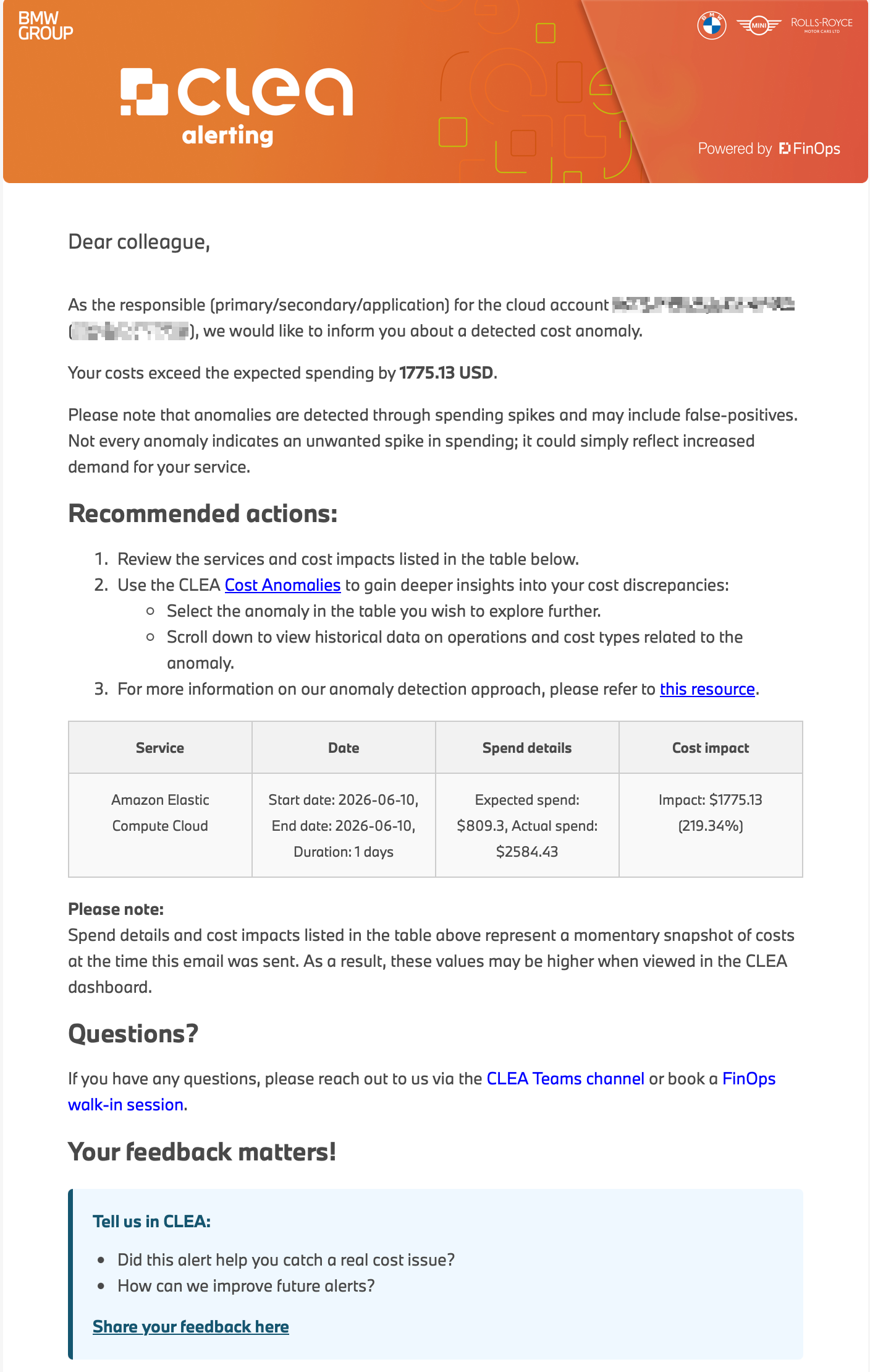
Figure 2: An anomaly alert as an account owner receives it
Self-service root cause analysis
When an alert lands, the owner can investigate without involving the platform team. CLEA provides an anomaly dashboard in Amazon Quick Sight that lists the detected anomalies for each account, using the same fields as the alert email. Owners can widen the filter to include anomalies that were not flagged for alerting, which is how borderline cases get reviewed.
When you select an anomaly, CLEA opens a drill-down chart. Two bar charts break the account’s actual daily spend down by operation and by usage type, which is usually enough to confirm the spike and place it in time. A detail table lists the usage types driving the cost, such as EUC1-InstanceUsage:db.r6g.large, with cost in US dollars and usage amount. In our own review of past cases, usage type and operation together accounted for the large majority of root causes, which is why the drill-down leads with those two dimensions.
Figure 3 shows the drill-down for an account with a confirmed spike. The left chart plots daily usage cost by operation from early May to mid-June 2026. RunInstances dominates, and a single day reaches about $2,600 against a baseline near $900. The right chart plots the same period by usage type, and the same day resolves almost entirely to EUC1-BoxUsage:g6.48xlarge, which identifies the instance type behind the spike.
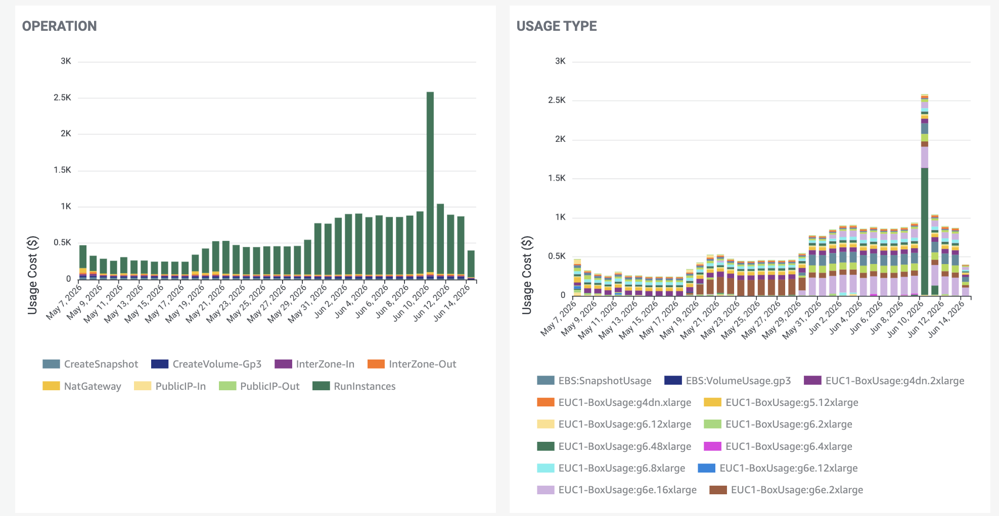
Figure 3: Daily cost by operation and by usage type for an account with a detected anomaly
Architecture and scale
The daily pipeline runs on AWS Step Functions in Distributed Map mode with a maximum concurrency of 500. Failure tolerance is set to five accounts out of roughly 14,000, which requires a 99.96 percent success rate per run. The full cycle finishes in about 20 minutes, and the whole setup costs around $50 per month in compute, or less than half a cent per account per month. Because every component is serverless, there is no idle infrastructure to pay for between runs.
Figure 4 shows the flow across three areas: the CLEA provider account, where dbt (data build tool) and the Step Functions workflow run. The Cloud Data Hub, which holds the raw, source, and semantic data layers together with the AWS Glue Data Catalog. And the CLEA dashboard, which reads a SPICE dataset in Amazon Quick Sight. The following numbered steps match the callouts in the diagram.
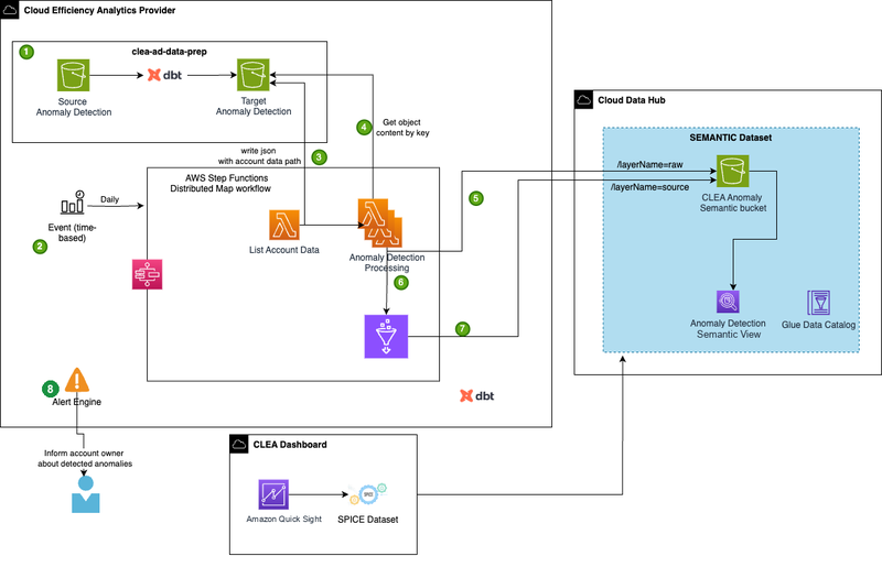
Figure 4: The daily anomaly detection pipeline
1. dbt repartitions the cost data into account-level Parquet files, one per account, aggregated per service per day.
2. A daily time-based event starts the Step Functions workflow.
3. The preparation Lambda function writes the account list to Amazon S3 as JSON.
4. Each Distributed Map worker reads its account’s data by key.
5. Workers write anomaly results to a raw Amazon S3 layer as one JSON file per account.
6. An AWS Glue job consolidates those files into a single daily Parquet file in the source layer.
7. Amazon Athena views expose the results, and the dbt models apply the threshold logic, range grouping, and alert labeling.
8. The alert engine reads the labeled output and sends the notifications.
Where CLEA goes next
The modular architecture positions CLEA to evolve its forecasting component as new time series models are released, without disrupting the downstream detection and alerting layers that account owners depend on daily.
Planned enhancements include integrating anomaly alerts with the existing IT service management (ITSM), so account owners receive incident tickets through workflows they already use daily rather than relying solely on email notifications.
On the self-service side, the team plans to give account owners direct control over their alert sensitivity through the CLEA recommendation management portal. Users will be able to define the total cost discrepancy that triggers a notification for their accounts, reducing reliance on centrally managed thresholds.
Further ahead, the team is building an agentic endpoint that will provide automated root cause explanations: what likely caused the spending increase, and what to do next to stop the anomaly or prevent it from recurring. The team also plans an AWS CloudTrail integration. It surfaces which user or role configured the service behind the cost increase, which adds configuration attribution to the remediation workflow.
Conclusion
We showed how BMW Group moved CLEA from reactive dashboards to daily, automated cost anomaly detection across more than 14,000 cloud accounts. For account owners, the practical change is that anomalies now come to them. Nobody has to remember to open a dashboard to learn that a service started costing more than it should, and because the alert lands the day after the spend occurs, owners can investigate while the cause is still fresh. A Prophet baseline per account-service pair supplies the expected spend. A layered set of filters reduces the raw detections to the ones worth an owner’s attention. A serverless pipeline on AWS Step Functions, AWS Lambda, AWS Glue, and Amazon Athena runs the whole cycle in about 20 minutes for roughly $50 per month. The part that took the most iteration was not the forecast. It was deciding which deviations deserve an email, and account owner feedback still drives how we tune those thresholds.
To build something similar, start with the Step Functions Distributed Map documentation for the fan-out pattern, and the AWS Cost and Usage Reports documentation for the billing data. For the rest of the CLEA story, see BMW Cloud Efficiency Analytics powered by Amazon Quick Sight and Amazon Athena on the data foundation and dashboards, How BMW Group built a serverless terabyte-scale data transformation architecture with dbt and Amazon Athena on the transformation layer beneath it, and How BMW Group Enhances Cloud Optimization With Generative AI on AWS on the assistant that BMW Group layered on top. If you would like help applying this pattern in your own organization, contact your AWS account team.
About the authors


