

# Introduction
We have given three similar interview questions from StrataScratch in SQL, Pandasand a Claude agent. Every piece of code is run against the same dataset, and each time number is the average over 500 runs. The agent's responses are exactly what Claude produces in response to written information, rather than a hypothetical example of what the agent might produce.
The comparison applies to all eight dimensions: speed, accuracy, definition, error correction, scalability, flexibility, risk of omission, and readiness for production. The three questions take the difficulty levels of easy, medium, and hard. The more complex the query, the more significant differences between SQL, Pandas, and agents become apparent.
# How We Ran This Comparison
The three questions come from the StrataScratch interview bank and cover easy, medium, and hard difficulty levels. SQL continued SQLite in memory, timed over 500 runs, the median is taken. Pandas worked on the same dataset Python 3.12, and over 500 runs. Claude's agent claude-sonnet-4-6called Anthropic API.
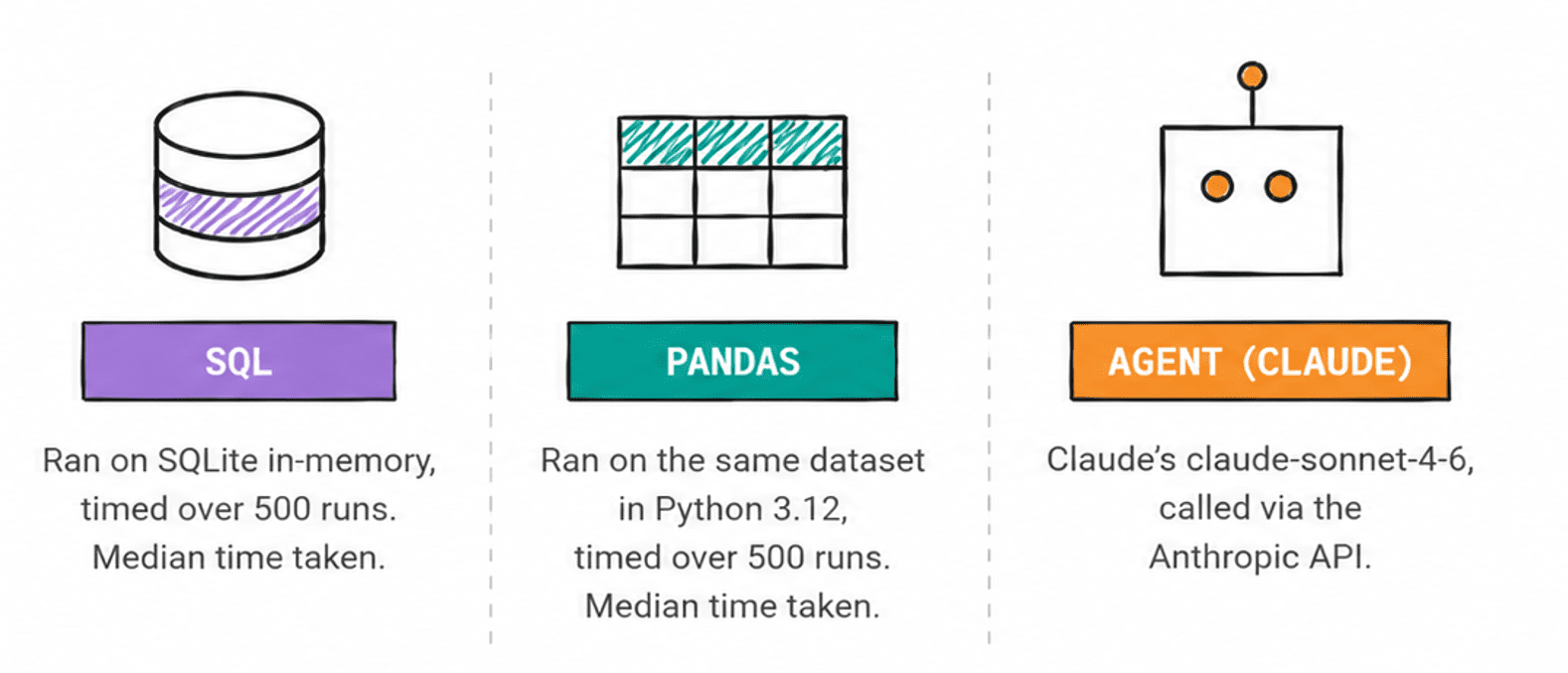
Each query has its own schema-based information that includes table names, column names, and a few sample rows. The system command below remains the same for all three calls. Agent response times are measured from the time a request is sent to the first token received.
# Simple Retrieval: All Three Agree
In the first interview question from Meta, users are asked to find every user who has done at least one scroll_up event and return unique user IDs. The data resides in a single table called facebook_web_log.
// The data
Here it is facebook_web_log the table.
| User ID | time stamp | action |
|---|---|---|
| 0 | 2019-04-25 13:30:15 | page_load |
| 0 | 2019-04-25 13:30:18 | page_load |
| 0 | 2019-04-25 13:30:40 | scroll_down |
| 0 | 2019-04-25 13:30:45 | scroll_up |
| … | … | … |
| 0 | 2019-04-25 13:30:40 | exit_page |
// SQL Coding Solution (0.002 ms)
SELECT DISTINCT user_id
FROM facebook_web_log
WHERE action = 'scroll_up';
// Pandas Coding Solution (0.40 ms)
import pandas as pd
result = (
    facebook_web_log[facebook_web_log['action'] == 'scroll_up']
    .drop_duplicates(subset="user_id")[['user_id']]
)
// Agent Prompt
Table: facebook_web_log (user_id INTEGER, action TEXT, timestamp TEXT)
Sample rows:
(1, 'scroll_up',   '2019-01-01 00:00:00')
(2, 'scroll_down', '2019-01-01 00:01:00')
(3, 'like',        '2019-01-01 00:03:00')
(2, 'scroll_up',   '2019-01-01 00:04:00')
Question: Find all users who performed at least one scroll_up event.
Return distinct user IDs.
// Agent output (2 seconds)
SELECT DISTINCT user_id
FROM facebook_web_log
WHERE action = 'scroll_up';
Output: All three return users 1 and 2.
In the single filter problem, the agent is exactly the same as SQL. The only real danger in this difficulty is naming the columns. Without the schema at the prompt, action may return as event_type or event_namereturning nothing and making no mistake.
# Multi-Step Integration: When Schema Grounding Matters
The second question is about product feature completion. The app tracks how far each user gets through a set of product features, where each feature has a fixed number of steps.
The task is to calculate the average completion percentage of each feature for all users, where the user's completion is their highest step reached divided by the number of steps for that feature, times 100. Users who never started a feature were counted as 0% completion.
Two tables feed this: facebook_product_features:
| attribute_identity | n_steps |
|---|---|
| 0 | 5 |
| 1 | 7 |
| 2 | 3 |
again facebook_product_features_realizations.
| attribute_identity | User ID | step_reached | time stamp |
|---|---|---|---|
| 0 | 0 | 1 | 2019-03-11 17:15:00 |
| 0 | 0 | 2 | 2019-03-11 17:22:00 |
| 0 | 0 | 3 | 2019-03-11 17:25:00 |
| 0 | 0 | 4 | 2019-03-11 17:27:00 |
| … | … | … | … |
| 1 | 1 | 3 | 2019-04-05 13:00:07 |
// SQL Coding Solution (0.007 ms)
WITH max_step AS (
    SELECT
        feature_id,
        user_id,
        MAX(step_reached) AS max_step_reached
    FROM facebook_product_features_realizations
    GROUP BY feature_id, user_id
),
calc_per_feature AS (
    SELECT
        feats.feature_id,
        n_steps,
        max_step_reached,
        COALESCE(max_step_reached, 0) * 1.0 / n_steps AS share_of_completion
    FROM facebook_product_features feats
    LEFT OUTER JOIN max_step
        ON feats.feature_id = max_step.feature_id
)
SELECT
    feature_id,
    AVG(share_of_completion) * 100 AS avg_share_of_completion
FROM calc_per_feature
GROUP BY feature_id;
// Pandas Coding Solution (2.05 ms)
import pandas as pd
# max step per user per feature
max_step = (
    facebook_product_features_realizations
    .groupby(['feature_id', 'user_id'])['step_reached']
    .max()
    .reset_index()
)

# join to features, fill users who never started with 0
df = pd.merge(
    facebook_product_features,
    max_step,
    how='outer',
    on='feature_id'
).fillna(0)

# completion % per user-feature row
df['share_of_completion'] = (df['step_reached'] / df['n_steps']) * 100

# average per feature
result = (
    df.groupby('feature_id')['share_of_completion']
    .mean()
    .to_frame('avg_share_of_completion')
    .reset_index()
)
// Agent Prompt
Tables:
- facebook_product_features (feature_id INTEGER, n_steps INTEGER)
- facebook_product_features_realizations
  (feature_id INTEGER, user_id INTEGER, step_reached INTEGER, timestamp TEXT)
Question: For each feature, calculate the average completion percentage
across all users. A user's completion = max(step_reached) / n_steps * 100.
Users who never started count as 0% completion.
Return: feature_id, avg_share_of_completion.
// Agent output (3 seconds)
WITH user_max_steps AS (
    SELECT feature_id, user_id, MAX(step_reached) AS max_step
    FROM facebook_product_features_realizations
    GROUP BY feature_id, user_id
)
SELECT
    f.feature_id,
    ROUND(AVG(COALESCE(ums.max_step, 0) * 100.0 / f.n_steps), 2) AS avg_share_of_completion
FROM facebook_product_features f
LEFT JOIN user_max_steps ums ON f.feature_id = ums.feature_id
GROUP BY f.feature_id
ORDER BY f.feature_id;
Output: All three return the same numbers.
| attribute_identity | completion_share_rate |
|---|---|
| 0 | 80 |
| 2 | 0 |
| 1 | 76.19 |
The agent got it here because the information said: “Users who have never started count as 0% completion. That expression is loaded. Without it, the agent writes an inner join – which drops non-starters – and the whole average goes up. That failure is silent. The numbers come back clean, and they are wrong. You will need to know the expected output to catch it.
# Multiple Tables and Window Concept: All Three Are Good, One is Too Slow
The third question covers Meta's data center energy consumption across the three regions. Each region has its own table: fb_eu_energy, fb_na_energyagain fb_asia_energy.
The function is to sum, the total usage by date, and produce two columns obtained: the active cumulative total and that total as a percentage of the total amount, rounded to the total amount.
// The data
Each state table has the same shape.
fb_eu_energy:
| recorded_date | use |
|---|---|
| 2020-01-01 | 400 |
| 2020-01-02 | 350 |
| 2020-01-03 | 500 |
| 2020-01-04 | 500 |
| 2020-01-07 | 600 |
fb_na_energy:
| recorded_date | use |
|---|---|
| 2020-01-01 | 250 |
| 2020-01-02 | 375 |
| 2020-01-03 | 600 |
| 2020-01-06 | 500 |
| 2020-01-07 | 250 |
fb_asia_energy:
| recorded_date | use |
|---|---|
| 2020-01-01 | 400 |
| 2020-01-02 | 400 |
| 2020-01-04 | 675 |
| 2020-01-05 | 1200 |
| 2020-01-06 | 750 |
| 2020-01-07 | 400 |
// SQL Coding Solution (0.010 ms)
WITH total_energy AS (
    SELECT recorded_date, consumption FROM fb_eu_energy
    UNION ALL
    SELECT recorded_date, consumption FROM fb_asia_energy
    UNION ALL
    SELECT recorded_date, consumption FROM fb_na_energy
),
energy_by_date AS (
    SELECT
        recorded_date,
        SUM(consumption) AS total_energy
    FROM total_energy
    GROUP BY recorded_date
    ORDER BY recorded_date ASC
)
SELECT
    recorded_date,
    SUM(total_energy) OVER (
        ORDER BY recorded_date ASC
    ) AS cumulative_total_energy,
    ROUND(
        SUM(total_energy) OVER (ORDER BY recorded_date ASC) * 100.0
        / (SELECT SUM(total_energy) FROM energy_by_date),
        0
    ) AS percentage_of_total_energy
FROM energy_by_date;
// Pandas Coding Solution (1.84 ms)
import pandas as pd
merged_df = pd.concat([fb_eu_energy, fb_asia_energy, fb_na_energy])

energy_by_date = (
    merged_df.groupby('recorded_date', as_index=False)['consumption']
    .sum()
    .sort_values('recorded_date')
)

energy_by_date['cumulative_total_energy'] = energy_by_date['consumption'].cumsum()
energy_by_date['percentage_of_total_energy'] = round(
    energy_by_date['cumulative_total_energy'] * 100 / energy_by_date['consumption'].sum()
)

energy_by_date['recorded_date'] = pd.to_datetime(
    energy_by_date['recorded_date']
).dt.strftime('%Y-%m-%d')

result = energy_by_date[
    ['recorded_date', 'cumulative_total_energy', 'percentage_of_total_energy']
]
// Agent Prompt
Tables:
- fb_eu_energy   (recorded_date TEXT, consumption INTEGER)
- fb_na_energy   (recorded_date TEXT, consumption INTEGER)
- fb_asia_energy (recorded_date TEXT, consumption INTEGER)
Question: Combine all three tables. Sum consumption by date. Output:
- recorded_date
- cumulative_total_energy (running sum across dates, ordered by date)
- percentage_of_total_energy (running cumulative / grand total * 100,
  rounded to the nearest whole number)
// Agent output (4 seconds)
WITH all_energy AS (
    SELECT recorded_date, consumption FROM fb_eu_energy
    UNION ALL
    SELECT recorded_date, consumption FROM fb_na_energy
    UNION ALL
    SELECT recorded_date, consumption FROM fb_asia_energy
),
daily_totals AS (
    SELECT recorded_date, SUM(consumption) AS daily_total
    FROM all_energy
    GROUP BY recorded_date
)
SELECT
    recorded_date,
    SUM(daily_total) OVER (ORDER BY recorded_date) AS cumulative_total_energy,
    ROUND(
        SUM(daily_total) OVER (ORDER BY recorded_date) * 100.0
        / SUM(daily_total) OVER (),
        0
    ) AS percentage_of_total_energy
FROM daily_totals
ORDER BY recorded_date;
Output: All three return the same table.
| recorded_date | cumulative_total_energy | percent_of_total_power |
|---|---|---|
| 2020-01-01 | 1050 | 13 |
| 2020-01-02 | 2175 | 27 |
| 2020-01-03 | 3275 | 40 |
| 2020-01-04 | 4450 | 55 |
| 2020-01-05 | 5650 | 69 |
| 2020-01-06 | 6900 | 85 |
| 2020-01-07 | 8150 | 100 |
The agent used SUM(daily_total) OVER () (window function with no ORDER BY) as a denominator instead of a scalar subquery in a SQL reference solution. Both methods work. The output is exactly the same.
# Three Comparisons
// Speed
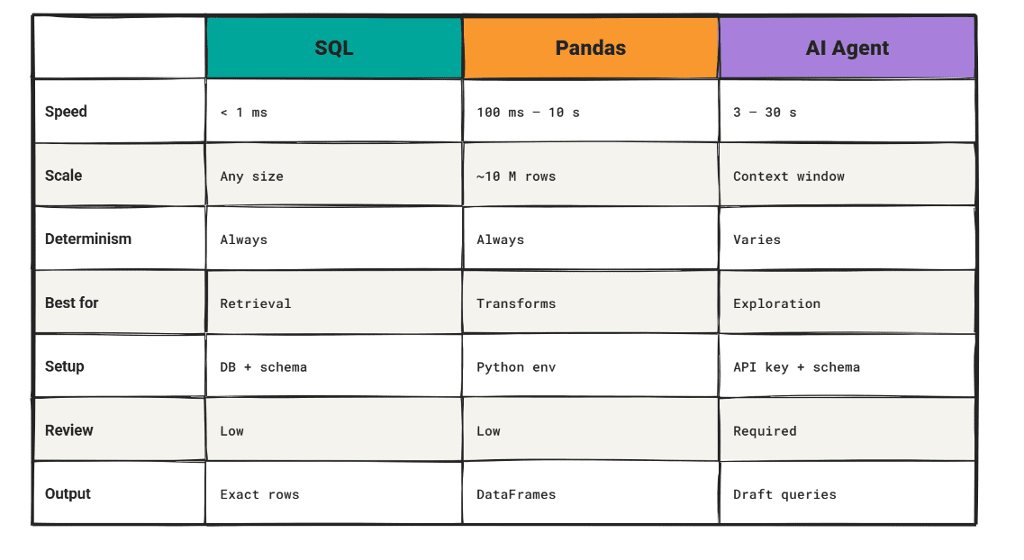
At this data scale, SQL ran at 0.002-0.010 ms, Pandas at 0.4-2.1 ms. The agent added 2-4 seconds of large language model (LLM) timeout before any SQL started.
The agent generates the code first; that generation time is the end of each query cycle. At warehouse scale, the gap closes to zero once the code is generated; SQL benefits further because it runs inside the database engine, and Pandas hits memory around 10 million rows and needs. Apache Spark or Timber beyond that.
// Accuracy and Risk of Hallucinations
SQL and Pandas are deterministic. The same code on the same data gives the same answer every time. With schema-based instructions, Claude got all three queries right, but each call produced different SQL names (different common table names (CTE), different column aliases, different but similar methods). Without a schema, the risk of hallucinations increases rapidly.
// Explanation and debugging
An SQL query is read in one block. A bad join situation appears in the text. Pandas requires Python fluently, but you can check it out DataFrame at each step. Agents explain their reasoning in English, and then display a code that you may or may not display. If the generated SQL is incorrect, you trace the error through the model's logic chain rather than reading the query you wrote.
// Flexibility and productivity readiness
Pandas is the clearest choice for custom transformations, branching, and iterative feature engineering. SQL handles logical setup cleanly and gets verbose for procedure work. Agents respond to requests in plain English, with very little consistency when the schemas are complex or ambiguous. For deployment, SQL is the most proven option for analytics; Pandas are experimentally reliable; and agents are trusted today with low-cost inquiries or when your output is reviewed before it starts.
# What Agent Results Really Show
With schema-based information, Claude got all three correct: Easy, Medium, and Hard. The SQL agent for the complex query used a different window operation pattern than the reference solution and still returned the correct table.
Two factors limit that finding. First, reproducibility: each API call can return different SQL for the same query. The concept is the same, but the team that reviews the queries generated by the agent needs to validate the output instead of hoping that the correct implementation will be the same as the next one. Second, it depends on the schema: the above commands include table and column names, as well as sample rows. Remove those, and the agent is guessing.
On easy difficulty, wrong guesses produce a null result. On Hard Difficulty, a wrong guess produces an unerringly wrong result.
A working pattern is: provide the full schema, invoke the SQL, then run and validate the output before it goes downstream.
# The conclusion
SQL, Pandas, and Claude each received three analytical queries when used correctly. The difference is in speed (0.01 ms vs 4 seconds), reproduction, and what happens when you drop the context.
SQL equates to structured retrieval and logic based on millisecond usage and deterministic output. Pandas equates to customized changes and a step-by-step notebook running on nearly 10 million lines. The agent suits the questions of the first draft and the interim evaluation, with a complete program in the notification and the person who reviews the output.

The agent got a tough question through SUM() OVER() instead of a scalar subquery, which is a valid option that the SQL index solution did not take. That's the honest version of this comparison: an agent can generate correct, intelligent SQL. It just adds a delay, it varies between runs, and it depends entirely on what you put in the notification.
Nate Rosidi he is a data scientist and product strategist. He is also an adjunct professor of statistics, and the founder of StrataScratch, a platform that helps data scientists prepare for their interviews with real interview questions from top companies. Nate writes about the latest trends in the job market, provides interview advice, shares data science projects, and covers all things SQL.


