
my series on Outlier Detection. In this article, we look at working with categorical data.
Generally when performing outlier detection with tabular data, we start by converting the data so that it is either entirely categorical or entirely numeric. There are some exceptions, but for the most part this is necessary: most outlier detection algorithms will assume the data is strictly in one format or the other, and we’ll need to get the data into the format the detector expects.
If the detector expects categorical data, the numeric features will need to be converted to a categorical format, which generally means binning them. And if the detector expects numeric data, any categorical features need to be numerically encoded. This is the more common scenario (the majority of outlier detection algorithms assume numeric data), and is what we’ll cover in this article.
Other articles in the series include: Deep Learning for Outlier Detection on Tabular and Image Data, Distance Metric Learning for Outlier Detection, An Introduction to Using PCA for Outlier Detection, Interpretable Outlier Detection: Frequent Patterns Outlier Factor (FPOF), and Perform Outlier Detection More Effectively Using Subsets of Features.
This article also covers some material from the book Outlier Detection in Python.
Outlier Detectors
Some examples of outlier detection algorithms that assume categorical data include: Frequent Patterns Outlier Factor (FPOF), Association Rules, and Entropy-based methods. Some that work with numeric data include: Isolation Forests, Local Outlier Factor (LOF), kth Nearest Neighbors (kNN), and Elliptic Envelope.
If you’re familiar with any outlier detection algorithms, it’s more likely the numeric algorithms, particularly Isolation Forest and LOF; these are probably the most commonly used algorithms. Further, all of the outlier detection algorithms included in scikit-learn and in PYOD (Python Outlier Detection) assume completely numeric data.
At the same time, the great majority of real-world tabular data is actually mixed (containing both numeric and categorical columns), which means, it’s very common when performing outlier detection to need to encode the categorical columns.
There is a reason for this: mixed data is more difficult to perform outlier detection on. Working with data of just one type (all categorical or all numeric) does simplify the work of finding the most unusual items in the data.
And, if we work with numeric data, we have the further benefit of being able to view the data geometrically: as points in space. If there are, say, 20 numeric columns in a table, then each row of the data can be viewed as a point in 20-dimensional space. At least, we can conceptually imagine them in 20-d space — the human mind can’t actually picture this. But we can picture 2d and 3d spaces and can extrapolate the general idea: we’re looking for points that are physically very distant from most other points. For example, in 2d, we may have data such as:
Here, we assume the data has just two features, called A and B, both with numeric values. Each row in the data is drawn either as a blue dot or a red star, with its location based on the values in the A and B columns. The blue dots indicate typical data, and the red stars represent a subset of the points that could be reasonably considered outliers: some points on the fringes of the clusters, and the points outside the clusters (the data has three main clusters, as well as some points outside these).
This is quite natural in lower dimensions. Things are different in high dimensions, due to what’s called the curse of dimensionality, and we do have to be mindful of that. But, conceptually, the idea of outliers as relatively isolated points in high-dimensional space is fairly straightforward.
Most numeric outlier detectors work by calculating the distances between each pair of points, and using these distances to identify the points that are most unusual — the points that have few points near them and that are far away from most other points. Though, in practice (for efficiency), the algorithms won’t actually calculate every pairwise distance (some can be skipped where it won’t substantially affect the outlier scores), but in principle, this is what the majority of numeric outlier detectors are doing.
We need, then, ways to convert categorical data to a numeric format that supports this well; that is, that makes it meaningful to calculate distances between rows after encoding the categorical values as numbers.
Methods to encode categorical data
With prediction problems, the most common encoding methods likely include:
- One-hot encoding
- Ordinal encoding
- Target encoding
With outlier detection, the set of options is a bit different, and the strengths and weaknesses of each are also different. Out of the three methods listed here, really only One-hot encoding works well for outlier detection. With outlier detection, the most effective are likely:
- One-hot encoding
- Count encoding
I’ll describe how each works, and why some work better than others for outlier detection. And I’ll explain why Count encoding (which is rarely used with prediction problems) can be quite useful with outlier detection.
I should also say, besides these encoding methods, there are several others that can be useful for prediction. An excellent library for encoding methods is Category Encoders. This will likely cover any of the methods you will need. Many of the methods provided, though, such as Target encoding and CatBoost encoding, require a target column, which is normally not available with outlier detection.
For example, if we had a table representing historical information about customers of a business, there may be a categorical column for “Last Product Purchased” and a target column called “Will Churn in next 6 Months”. The “Last Product Purchased” column may have the distinct values: “Product A”, “Product B”, and “Product C”. To encode these, we can calculate how often the target column has value True for each value (in the training data), possibly encoding these as 0.12, 0.43, 0.02 (meaning, when the ‘Last Product Purchased’ is Product A, 12% of the time the Target column is True, and the client churns in the next 6 months; similarly for Product B (43%) and Product C (2%)).
But with outlier detection, we’re working in a strictly unsupervised environment: there is no ground truth value for how outlierish each row is, and so no way to set a Target column. We can use only unsupervised encoding methods, including One-hot and Count encoding.
One-hot encoding
To look at One-hot encoding, I’ll start by describing how it is done, and then will look at how it works with distance calculations. Let’s assume we start with a table such as the following:
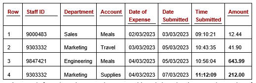 Table 1: Staff Expenses table
This table describes staff expenses, with one row per expense claim. Assuming we plan to use one or more numeric outlier detectors, we’ll need to convert the categorical columns (Staff ID, Department, and Account) to numbers.
The Date and Time columns will also need to be converted to numeric values. Outlier Detection in Python covers working with date and time data. I don’t have space in this article, but will say quickly that they can be converted in a number of ways. One simple method is by calculating the time since some starting point (referred to as the epoch). The minimum date or time in the column may be used, or some other date that represents a logical starting point.
Let’s say we use January 1, 1990. All dates can then be represented as the number of days since that point. We do, though, also wish to capture more information about the dates, such as the day of the week (this may be relevant, for example, if staff expenses for weekends are unusual), if they fall on a holiday, and so on, so we may wish to look at other encoding methods as well. For this article, though, we’ll focus just on categorical columns.
If we consider, for the moment, just the Department column, by One-hot encoding this column, we replace the column with a series of new columns, one for each unique value in the column. Let’s assume the column had five distinct values: Sales, Marketing, Engineering, HR, and Communications. We would then have five new columns representing these values, such as in the following table (Table 2). This shows just the Staff ID column, and the new columns related to Department. (The other columns would be present as well, but are skipped here for simplicity. A similar set of columns would be created, for example, for the Account column).
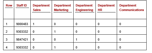 Table 2: Staff Expenses table with the Department column one-hot encoded (some columns not shown)
Each of the cells in the one-hot Department columns will have a value of either 0 or 1, indicating if that is the correct value for this row. We see here in the first row, an expense claim for Staff 9000483, who is in Sales. Given that, the column for ‘Department Sales’ has a 1 and the other columns related to the Department have a 0. Similarly, for each other row: exactly one of the Department columns will have a 1, and all others a 0.
One-hot encoding is very commonly used for outlier detection and can be a good choice when a feature has low cardinality. It can, though, break down somewhat where the column has very high cardinality. For example, if the Department column in the original staff expenses table had 100 distinct values, it would result in 100 new columns being created, which can create a table that’s difficult to work with. I’ll show below, though, that it’s actually no worse for distance calculations than with low-cardinality situations, and so may still be workable.
At the same time, high-cardinality columns are not generally as useful for outlier detection as low-cardinality columns. For this reason, we may not want to include the Staff Id column in the our outlier detection process. Though we also may: it may still be informative and useful to include — for example, if we wish to find expenses that are large for that staff, staff that have unusual numbers of expenses, staff that have many similar expenses close in time and so on.
One-hot encoding with Isolation Forest
How much of a problem generating many additional columns depends on the outlier detection algorithm. One of the most well-used outlier detection algorithms is Isolation Forest, which does not use distance calculations. Instead, it identifies low-density subspaces in the feature space and flags the rows that appear in these. Which means, it’s still looking for points that are far from other points, but does so without calculating the distances between points.
I can’t get into the details of Isolation Forest here (hopefully a future article, though), but will say quickly that if a single column is expanded into many columns after encoding (as with One-hot encoding and some other encoding schemes), those columns will be overrepresented in the analysis of the Isolation Forest algorithm, which we probably don’t want.
Due to some interesting details of how the Isolation Forest algorithm works internally, it’s actually usually most effective with Isolation Forests to use Ordinal encoding. Having said that, Isolation Forest is one of the very few outlier detection algorithms where this is true — with most other detectors Ordinal encoding works quite poorly. I’ll describe it below and explain why that’s the case.
Distance calculations with One-hot encoding
Most numeric outlier detectors, however, are based on calculating and assessing the distances between points (or between each point and the data center, or cluster centers). This includes: Local Outlier Factor, k-Nearest Neighbors, Radius, Gaussian Mixture Models, KDE (Kernel Density Estimation), Elliptic Envelope, One-Class Support Vector (OCSVM), and numerous others.
The encoding method will affect the distances calculated, and consequently, the outlier scores given to each row. One-hot encoding does usually work relatively well with outlier detection for most numeric detectors (including those based on distance calculations), but it does have one negative: as with Isolation Forests, One-hot encoding results in categorical features being overrepresented in distance calculations, though the effect is less severe than with Isolation Forests.
As an example, consider the following table (Table 3), which shows a dataset with four rows and two features. The Colour column has five values (with two present in the current data) — red, blue, green, white, and yellow. The size column has two values: big and small.
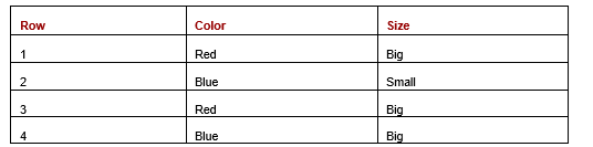 Table 3: Dataset with Colour and Size features
The pair-wise distances between the four rows are shown in the next table (Table 4). There are many distance calculations we could use; this method leaves the data as categorical (we don’t do any numeric encoding yet) and measures the distance between two rows as the number of values that are different.
As there are two features, a pair of rows can have a distance of zero, one, or two (they can have zero, one, or both features different). The table shows only the distances between each unique pair of rows and shows each distance only once (e.g. between Row 1 and Row 2, but between Row 2 and Row 1, which would be the same; and not between Row 1 and itself), so shows values only above the main diagonal.
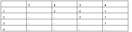 Table 4: Distances between each pair of rows using a distance metric that considers if features have the same value or not.
If we One-hot encode the original data (from Table 3), we get:
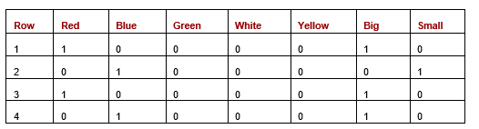 Table 5: Dataset after one-hot encoding
If we calculate the pair-wise distances between the rows using one-hot encoding and either Manhattan or Euclidean distances, we have the distances shown in the next table. In this case, as all values are 0 or 1, the Manhattan and Euclidean distances are actually the same.
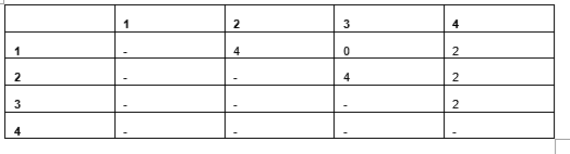 Table 6: Pairwise Manhattan/Euclidean distances
Using Manhattan (or Euclidean) distance measures, the distances are proportional to when using a count of the number of values matching (as we did for Table 4), but the values are double: when two values in the original data mismatch, there will be two cells in the one-hot encoding mismatched. This is not usually a problem when working with purely categorical data, but it does create an undesirable situation where we have mixed data.
Consider Table 7 with two features: Color and Weight, where Weight is numeric.
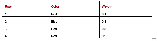 Table 7: Dataset with one categorical and one numeric feature
Once one-hot encoded, we have Table 8:
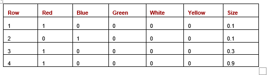 Table 8: One-hot encoding with one categorical and one numeric feature
Here, when we calculate Euclidean distances between the rows. (We can also use Manhattan, Canberra, or any other distance metric, but for this example, use Euclidean). We show the Euclidean distances in the following table (Table 9):
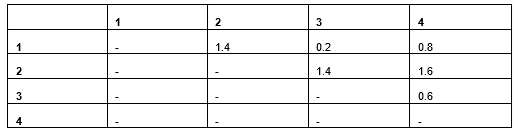 Table 9: Distances based on Euclidean distances
Rows 1 and 2 differ in the Colour (having the same weight) and have a Euclidean distance of 1.4. Rows 3 and 4 are different in weight (having the same color) and have a Euclidean distance of just 0.6. We can see the difference in Colour is more significant than Weight in determining the distance, though likely it should not be.
There are two factors that give categorical features more importance here than numeric. The first is that matches versus non-matches affect two one-hot columns, while the differences in numeric values affect only a single column. The second is that distances in binary columns are larger than in numeric features. Here, Row 1 and Row 4 have Weight values of 0.1 and 0.9, which have a significant difference of 0.8 — but this is less than the difference in two mismatching categorical values, which will be 2.0 (given that two binary columns will mismatch).
An example working with Manhattan and Euclidean distances is shown in the following listing. In the first case, we create a pair of vectors representing the first two rows from the previous data, with five one-hot columns for Colour and one column for Weight. We then create another pair of vectors to simulate what it would look like if the cardinality of Color were instead 2, using only two binary columns.
Here we show some code testing the Manhattan and Euclidean distances:
from sklearn.metrics.pairwise import euclidean_distances,
manhattan_distances

# Creates data simulating two rows where five binary columns are
# used for one categorical
row_1 = [1, 0, 0, 0, 0, 0.1]
row_2 = [0, 1, 0, 0, 0, 0.1]
print(manhattan_distances([row_1], [row_2]))
print(euclidean_distances([row_1], [row_2]))

# Creates similar data but with two binary columns for one
# categorical column
row_1 = [1, 0, 0.1]
row_2 = [0, 1, 0.2]
print(manhattan_distances([row_1], [row_2]))
print(euclidean_distances([row_1], [row_2]))
Interestingly, in both cases, the two rows have a Manhattan distance of 2.1 and Euclidean of 1.4: where we test using only two binary features for Colour instead of five, the distances are the same. Similarly, increasing the cardinality (using more than five binary columns to represent color) does not affect the distance measures. Regardless of how many one-hot columns there are related to Colour, if two rows have the same colour, there will be 0 differences; and if they have different colours, there will be 2 differences (all other columns will be zero, and therefore matching).
So, there is, as noted, an imbalance between categorical and numeric features, but it is not made worse by the cardinality of the categorical features.
My suggestion, to reduce the over-emphasis in distance calculations, is to replace the 1.0 values in the one-hot columns with 0.25. This will result in rows with different values having a total difference (with respect to that original column) of 0.5 instead of 2.0, putting it more in the same scale as the numeric features.
Ordinal encoding
Ordinal encoding works by simply giving each unique value in a categorical column a unique number. In the example above, we may give the values in the Colour column values such as:
red: 1
blue: 2
green: 3
white: 4
yellow: 5
So all values of “red” would be replaced by 1, and so on. Similarly for the Size column: we can replace ‘small” with, say, 1 and “big” with 2, or with any other numeric values.
As indicated, this does actually work well for Isolation Forest. But it doesn’t tend to work well for most other numeric outlier detectors, including those based on distances. Ordinal encoding does avoid creating additional columns: each categorical column is translated into a single numeric column. But, the distance calculations will become meaningless.
Using the values above, rows with value yellow would be considered 4.0 away from those with value red, while those with value white would only be 1.0 away from rows with yellow, which make little sense. The distances end up completely arbitrary.
Count encoding
Count encoding is actually much more important as an encoding technique with outlier detection than with prediction. As with Ordinal encoding, it coverts each categorical column to a single numeric column, but with Count encoding, does so in a way that the numeric values aren’t random; they have meaning, and meaning that’s relevant to outlier detection.
Count encoding also produces numeric values that are straightforward for distance calculations.
With Count encoding, the numeric values generated represent the frequency of the value (rare values will be given small values and common values large values), which has some real information value when working with outlier detection.
Taking a look at the Staff Expenses table, if we have a distribution of Department values such as:
Sales: 1,000
Marketing: 500
Engineering: 100
HR: 10
Communications: 3
Then, these counts will be the encodings. That is, 1,000 records (those for Sales) will be given value 1,000; 500 will have value 500; and so on. This has the advantage that it can encode values such that rare values tend to be far from other values. In this case, the values 10 and 3 are close to each other, which means these 13 records will be close to each other, but there are still only 13 of them, and they will be far from the other 1,600 records. The value 1,000 is distant from the other values, but there are 1,000 records with this encoding, and so these 1000 records are each close to 999 others, and would then not be flagged as outliers.
In the following code, using these values, we generate a simple, single-feature dataset representing the department and create a Local Outlier Factor (LOF) detector to assess this. When working with multiple columns, it is necessary to scale any Count-encoded features to ensure all features are on the same scale, but as this example contains only a single feature, this step may be skipped. The LOF is able to correctly identify the rare values as outliers: the 13 rare values are given prediction –1 (indicating outliers in the scikit-learn implementation), while all others are predicted as 1 (indicating inliers).
import numpy as np
import pandas as pd
from sklearn.neighbors import LocalOutlierFactor

# Creates a dataset with a single categorical column
vals = np.array(['Sales']*1000 + ['Marketing']*500 + ['Engineering']*100 +
['HR']*10 + ['Communications']*3)

# Count-encode the column
df = pd.DataFrame({"C1": vals})
vc = df['C1'].value_counts()
map = {x:y for x,y in zip(vc.index, vc.values)}
df['Ordinal C1'] = df['C1'].map(map)

# Uses LOF to determine the outliers in the column
clf = LocalOutlierFactor(contamination=0.01)
df['LOF Score'] = clf.fit_predict(df[['Ordinal C1']])
One thing to note about Count encoding is that it can give multiple original values the same numeric code if they happen to have the same count. For example, if Sales and Marketing both had 1000 rows, they would both be given an encoding of 1000. Or if Sales had 1000 and Marketing had 1001, they would be given nearly the same encoding. For most detectors, this is not an issue, but again, Isolation Forest is a bit different and it’s better to be able to distinguish values that actually are distinct, which is possible with Ordinal encoding.
Determining the best encoding method
Which encoding method works best will vary based on the dataset, the outlier detection algorithm, and the types of outliers you wish to find. Unfortunately, like many things in data science, there is no definitive answer as to what’s best; each method can be preferred at times. And, in some cases, it may actually work best to use different encodings for different features.
As is a common theme with outlier detection, it can be useful to take an ensemble approach, where rows are encoded in multiple ways. The truly anomalous rows will stand out as outliers using each encoding method, while the more mildly anomalous will possibly stand out just using one or another encoding method.
Choosing an encoding method can be easier with prediction problems. With prediction problems, we usually have a validation set and can simply try different encoding methods and determine experimentally which works best. With outlier detection, though, the problems are usually completely unsupervised (again, there is no target column as there is no ground truth as to how outlierish each row is). Which means it’s more difficult to evaluate the encoding methods used. We can, though, use a technique for evaluating outlier detection systems known as Doping.
As well, where the outlier detection system runs over time, it may be possible to collect labeled data and use this to evaluate different preprocessing methods including the encoding of the categorical columns.
Scaling
If we were working with data that was completely numeric to start with, we wouldn’t need to encode any categorical columns, but we would still need to scale the data, at least with most numeric outlier detectors. Again, Isolation Forest is one of the exceptions, but any based on distance calculations do require that each dimension (each feature) is on the same scale. Otherwise the distances between points (or between the points and cluster centers, etc.) will be dominated by features that happen to be on larger scales.
The same is true for any categorical columns after encoding. Regardless of the encoding method used, the new numeric features may now be on different scales than the features that were already numeric (and the converted date or time features). And, if different encoding methods are used for different categorical columns, then even these columns may be on different scales as each other.
Scaling these columns uses the same methods as numeric columns — we just have to ensure we include these new columns. The specifics of doing this will hopefully be covered in a future article, but quickly: we usually use either a min-max, robust z-scaling, or spline scaling for this.
All images were by the author


