
# Introduction
You probably typed a question into the search bar and got results that matched your words but missed your meaning entirely. Or watch a recommendation engine come up with something surprisingly valuable even though you never searched for it directly. The gap between “finding the exact words” and “understanding what someone really means” is what makes a search feature useful.
Vector search it fills that gap by representing text as points in a high-dimensional space, where geometric proximity encodes semantic similarity. Two sentences can share zero words and end up being neighbors because the model has learned that their meanings are close.
This article builds a vector search engine from scratch in Python using only NumPyto see exactly what happens at each step: how the embedding is preserved and normalized, why cosine similarity reduces to the dot product, and what the resulting search space actually looks like when you map it down to two dimensions.
You can find the code on GitHub.
# What is Vector Search?
Traditional keyword searches look for exact word matches. Vector search works in a different way: it converts documents and queries into numerical vectors called embeddings, and finds the closest vectors in a high-dimensional space.
The important understanding is that closeness in vector space means semantic similarity. Two sentences that mean the same thing – even if they don't match in words – will have close embeddings.
The distance metric you use to measure “closeness” is what drives the entire system. The most common is cosine symmetry, which measures the angle between two vectors rather than their absolute distance. This makes it flexible – useful if you care about direction or definition rather than size or word count.
# Sets the DataSet
We will work with a set of short product descriptions from a fictional e-commerce catalog. These are pre-embedded as 8-dimensional vectors – a much reduced dimension realistic enough to demonstrate concepts.
In a real system, you can generate this embedding from a model like sentence modifiers. In this tutorial, we simulate that step with controlled random data with a clear cluster structure.
import numpy as np

np.random.seed(42)

# Product catalog — 3 semantic clusters: electronics, clothing, furniture
products = [
    "Wireless noise-cancelling headphones with 30-hour battery",
    "Bluetooth speaker with waterproof design",
    "USB-C hub with 7 ports and power delivery",
    "4K HDMI cable 6ft braided",
    "Mechanical keyboard with RGB backlight",
    "Men's slim-fit chino pants navy blue",
    "Women's merino wool turtleneck sweater",
    "Unisex running jacket lightweight windbreaker",
    "Leather chelsea boots for men",
    "Organic cotton crew neck t-shirt",
    "Solid oak dining table seats 6",
    "Ergonomic mesh office chair lumbar support",
    "Linen sofa 3-seater natural beige",
    "Bamboo bookshelf 5-tier adjustable",
    "Memory foam mattress queen size medium firm",
]

# Simulate embeddings with cluster structure
# Cluster centers in 8D space
electronics_center = np.array([0.9, 0.1, 0.2, 0.8, 0.1, 0.3, 0.7, 0.2])
clothing_center    = np.array([0.1, 0.8, 0.7, 0.1, 0.9, 0.2, 0.1, 0.8])
furniture_center   = np.array([0.2, 0.3, 0.9, 0.2, 0.1, 0.9, 0.3, 0.1])

n_per_cluster = 5
noise = 0.08

embeddings = np.vstack([
    electronics_center + np.random.randn(n_per_cluster, 8) * noise,
    clothing_center    + np.random.randn(n_per_cluster, 8) * noise,
    furniture_center   + np.random.randn(n_per_cluster, 8) * noise,
])

print(f"Embeddings shape: {embeddings.shape}")
Output:
Embeddings shape: (15, 8)Each row is a product. Each column has one dimension for its embedding. Product names will not be used by search engines; only embedding matters.
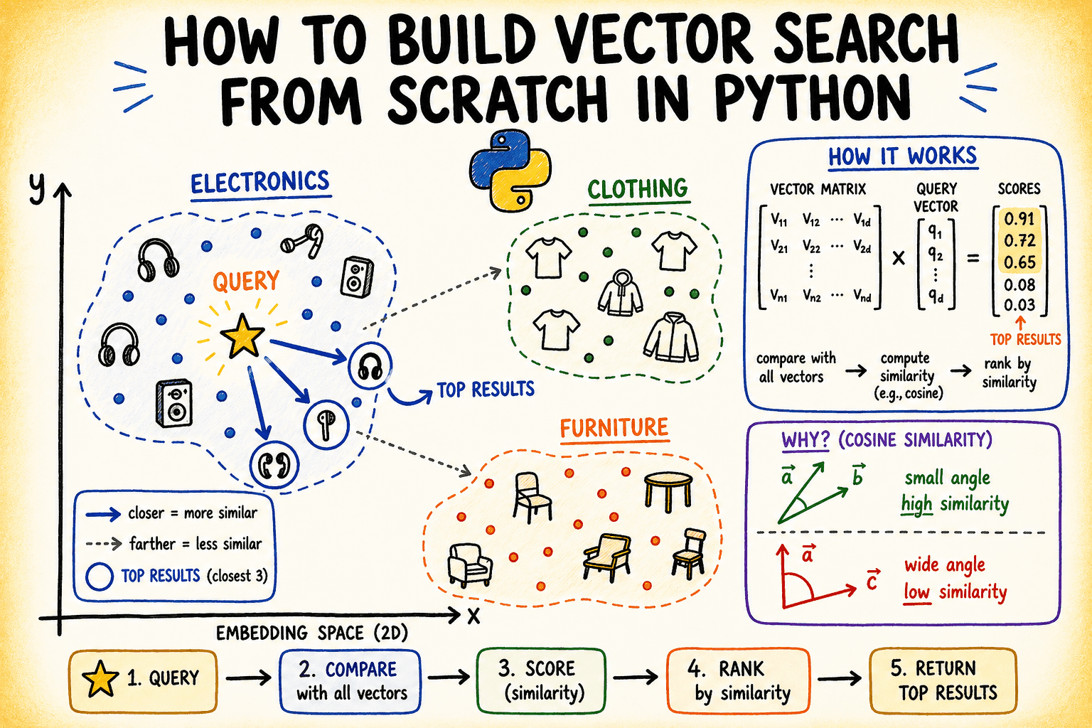
Photo by the Author
# Creating an Index
An “index” in a vector search engine is simply a stored set of standard embeddings. The normalization is important here because it makes the cosine similarity equal to the dot product, which is cheap to calculate.
def normalize(vectors: np.ndarray) -> np.ndarray:
    """L2-normalize each row vector."""
    norms = np.linalg.norm(vectors, axis=1, keepdims=True)
    # Avoid division by zero
    norms = np.where(norms == 0, 1e-10, norms)
    return vectors / norms

class VectorIndex:
    def __init__(self):
        self.vectors = None
        self.labels = None

    def add(self, vectors: np.ndarray, labels: list):
        self.vectors = normalize(vectors)
        self.labels = labels
        print(f"Indexed {len(labels)} items with {vectors.shape[1]}-dimensional embeddings.")

    def search(self, query_vector: np.ndarray, top_k: int = 3):
        query_norm = normalize(query_vector.reshape(1, -1))
        # Cosine similarity = dot product of normalized vectors
        scores = self.vectors @ query_norm.T  # shape: (n_items, 1)
        scores = scores.flatten()
        # Get top-k indices sorted by descending score
        top_indices = np.argsort(scores)[::-1][:top_k]
        return [(self.labels[i], float(scores[i])) for i in top_indices]

index = VectorIndex()
index.add(embeddings, products)
Output:
Indexed 15 items with 8-dimensional embeddings.I search method does three things: normalizes the query, calculates dot products against the entire stored vector, then sorts by score and returns the top-k results. That matrix multiplication (self.vectors @ query_norm.T) is the entire retrieval step.
# Running Quiz
Now let's test what we've built with a few questions. We construct the query vectors by starting at one of the cluster centers and adding some noise to simulate the real query embedding.
def make_query(center: np.ndarray, noise_scale: float = 0.05) -> np.ndarray:
    return center + np.random.randn(8) * noise_scale


queries = {
    "audio equipment": make_query(electronics_center),
    "casual wear":     make_query(clothing_center),
    "home furniture":  make_query(furniture_center),
}

for query_name, q_vec in queries.items():
    print(f"nQuery: '{query_name}'")
    results = index.search(q_vec, top_k=3)
    for rank, (label, score) in enumerate(results, 1):
        print(f"  {rank}. [{score:.4f}] {label}")
Output:
Query: 'audio equipment'
  1. [0.9856] Wireless noise-cancelling headphones with 30-hour battery
  2. [0.9840] USB-C hub with 7 ports and power delivery
  3. [0.9829] Mechanical keyboard with RGB backlight

Query: 'casual wear'
  1. [0.9960] Men's slim-fit chino pants navy blue
  2. [0.9958] Leather chelsea boots for men
  3. [0.9916] Women's merino wool turtleneck sweater

Query: 'home furniture'
  1. [0.9929] Bamboo bookshelf 5-tier adjustable
  2. [0.9902] Linen sofa 3-seater natural beige
  3. [0.9881] Solid oak dining table seats 6
Scores close to 1.0 indicate a nearly identical position in the embedding environment, which is exactly what you would expect from queries created from the same collection center as their target documents.
# Visualizing the Embedding Space
High-dimensional data is hard to think about visually. Principal component analysis (PCA) projects 8-dimensional embedding down to 2D so that we can see cluster structure. We will run a small PCA using only NumPy.
The following code compiles the 2D PCA projection and organizes all product embeddings by cluster labels and colors:
import matplotlib.pyplot as plt
import matplotlib.patches as mpatches

projected = pca_2d(embeddings)

cluster_colors = (
    ["#4A90D9"] * 5 +   # electronics — blue
    ["#E8734A"] * 5 +   # clothing — orange
    ["#5BAD72"] * 5     # furniture — green
)
cluster_labels = ["Electronics"] * 5 + ["Clothing"] * 5 + ["Furniture"] * 5

fig, ax = plt.subplots(figsize=(6, 4))
ax.scatter(projected[:, 0], projected[:, 1],
           c=cluster_colors, s=100, edgecolors="white", linewidths=0.7, zorder=3)
This part projects queries for vectors in the same space, overlays them, and completes the plot:
# Plot query projections
q_projected = pca_2d(
    np.vstack(list(queries.values())) - embeddings.mean(axis=0)
)
for (qname, _), (qx, qy) in zip(queries.items(), q_projected):
    ax.scatter(qx, qy, marker="*", s=200, color="gold",
               edgecolors="#333", linewidths=0.6, zorder=4)
    ax.annotate(f"⟵ query: {qname}", (qx, qy),
                textcoords="offset points", xytext=(6, -8),
                fontsize=7, color="#555555", style="italic")

legend_patches = [
    mpatches.Patch(color="#4A90D9", label="Electronics"),
    mpatches.Patch(color="#E8734A", label="Clothing"),
    mpatches.Patch(color="#5BAD72", label="Furniture"),
    mpatches.Patch(color="gold",    label="Query vectors"),
]
ax.legend(handles=legend_patches, loc="upper left", fontsize=6)
ax.set_title("Vector Search — Embedding Space (PCA projection)", fontsize=10, pad=10)
ax.set_xlabel("PC 1"); ax.set_ylabel("PC 2")
ax.grid(True, linestyle="--", alpha=0.4)
plt.tight_layout()
plt.savefig("embedding_space_queries_only.png", dpi=150)
plt.show()
Output:
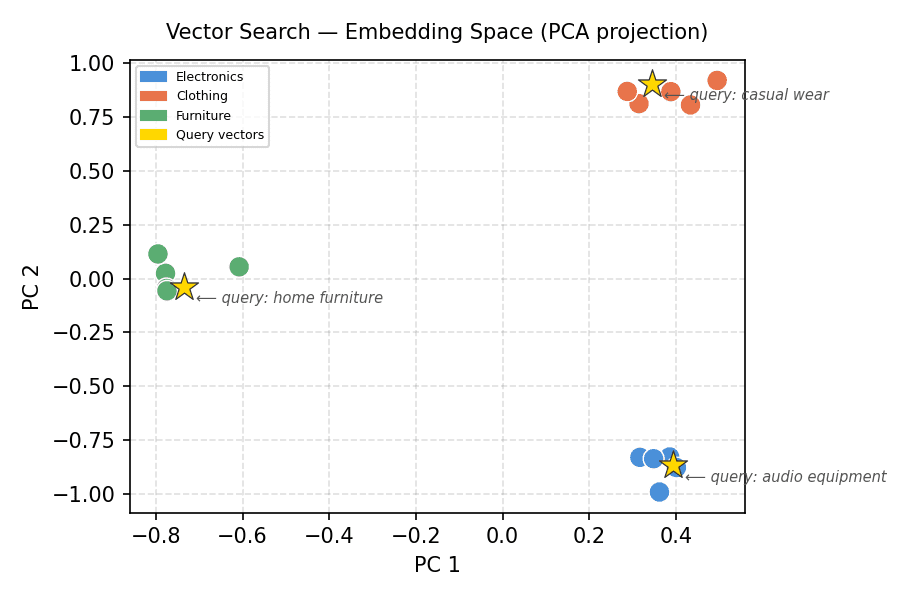
Vector Search – Embedding Space (PCA projection)
Clusters separate cleanly. Each gold star (query vector) resides within the cluster from which it is composed. This is the geometry that vector search uses.
# Visualizing Uniform Score Distributions
For any given query, it's useful to see how similar scores are distributed throughout the index – and not just in the top-k. This tells you whether the top score is the clear winner or slightly better than the rest.
q_vec_furniture = queries["home furniture"]
q_norm_furniture = normalize(q_vec_furniture.reshape(1, -1))
all_scores_furniture = (index.vectors @ q_norm_furniture.T).flatten()

sorted_idx_furniture = np.argsort(all_scores_furniture)[::-1]
sorted_scores_furniture = all_scores_furniture[sorted_idx_furniture]
sorted_labels_furniture = [products[i][:30] + "…" if len(products[i]) > 30
                           else products[i] for i in sorted_idx_furniture]

# Define bar colors: green for furniture items, gray for others
bar_colors_furniture = []
for i in sorted_idx_furniture:
    if i >= 10 and i <= 14:  # Furniture items are originally at indices 10-14
        bar_colors_furniture.append("#5BAD72") # Green for furniture
    else:
        bar_colors_furniture.append("#cccccc") # Gray for others

fig, ax = plt.subplots(figsize=(10, 5))
bars = ax.barh(sorted_labels_furniture[::-1], sorted_scores_furniture[::-1],
               color=bar_colors_furniture[::-1], edgecolor="white", height=0.65)

ax.axvline(sorted_scores_furniture[2], color="#5BAD72", linestyle="--",
           linewidth=1.2, label="Top-3 cutoff")
ax.set_xlim(sorted_scores_furniture.min() - 0.002, 1.001)
ax.set_xlabel("Cosine Similarity Score")
ax.set_title("Query: 'home furniture' — Similarity Across All Products", fontsize=11, pad=12)
ax.legend(fontsize=8)
ax.grid(axis="x", linestyle="--", alpha=0.4)
plt.tight_layout()
plt.savefig("score_distribution_furniture.png", dpi=150)
plt.show()
Output:
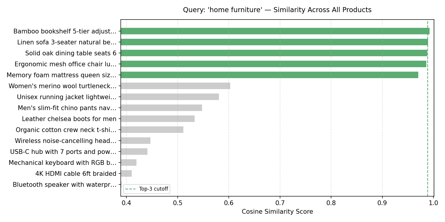
Question: 'home furniture' — Similarities Across Brands
There is a noticeable gap between the furniture collection (top 5 bars) and everything else. Basically, you will use this gap to set the same limit below when the results are completely compressed.
# Wrapping up
He built a vector search engine with about 50 lines for NumPy: an index class that normalizes and stores embeddings, a search method that uses matrix multiplication to calculate cosine similarity, and two visualizations that display the geometry behind the results.
The next step is to replace the simulated embed with the original. Try loading sentence converters and embedding your text corpus. The reference code here will work without changes.
If you'd like to read more “from scratch” articles, let us know what you'd like to see next!
Count Priya C is an engineer and technical writer from India. He loves working at the intersection of mathematics, programming, data science, and content creation. His areas of interest and expertise include DevOps, data science, and natural language processing. She enjoys reading, writing, coding, and coffee! Currently, he works to learn and share his knowledge with the engineering community by authoring tutorials, how-to guides, ideas, and more. Bala also creates engaging resource overviews and code tutorials.


")
