To assess the appropriateness of the eligibility and an attack on ATOTIONS costs that call the epython turn

The objectives of the temperature of 1.5 ° C by the end of the age of Paris, various institutions arise with various circumstances. There is a contract between reducing the minimum and low technology.

The submission of the reduction technology options (such as renewable energy, electric cars, green hydrogen, etc.) Come with their costs and benefits. The integration of renewable power and fatty oils in Portofofolio electricity is not only determining the CO2 but may affect the price of electricity. In this post, I will discuss how the price of electricity is determined in a complete electricity market with Merit Order Curve (Based on the thought of Costside cost or production), and that the effectiveness of the costs of decalechons or district or organization may be evaluated based on the The risk of risk costs a curve. I will use the Python to form these two curves, and discuss the implementation.

Let's get started!

Merit Order Curve

The electrician or national use may have the competitive energy plants of different types of portfolio to provide electricity from the merchants. This is known as a complete electricity market (also known as the Spot Market). The cost of generating electricity vary in the type of power center. For example, there are a romantic or small cost of electricity from the solar PV or air turbines because they do not need any oil. On the other hand, Fossil oil plants have higher high costs in accordance with electricity prices such as coal, oil, or combined gas to produce electricity. In economic, the cost of producing one additional unit of product is called Marginal cost of manufacturing. Based on the rising edition of the back cost of the simple runs of electricity production. This sequence is called advice. Martial Randard Plans are organized to meet the need first, followed by power plants with the right side of the expansion of the provision of electricity.

At this stage, I will use different steps to build a Merit Order Epython turn and discuss how the Merit order sets electrical electrical price.

Work

Let's see that there are nine-kinds plants for a portfolio of the country as shown in the list power_plants. These energy plants must be organized by the rise of marginal_costs. Information used in this example is based on my thinking and can be considered as dummy details.

power_plants = ["Solar", "Wind", "Hydro", "Nuclear", "Biomass", "Coal", "Gas", "Oil", "Diesel"]

marginal_costs = [0, 0, 5, 10, 40, 60, 80, 120, 130]

First, I convert this data to the dataframe with power_plants direct marginal_cost to the column. Next, I use the data data index and ask the user to install the available dose of energy plant. Available capacity of each plant is kept in the variety of individuals using globals() method as shown below.

^{The user's entries to find the available volume of Power Prep each using LOOP and the Globals () the way.}

The total number of existing Portfolio X reaches 1800 MW. Then, I am creating a new column called Cumulative capacity (MW)which is a compound value of this Available capacity (MW) .

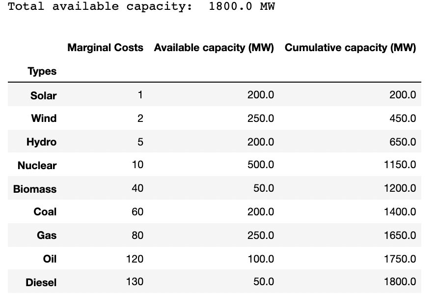
^{The dataframe contains the side cost and the available power for the Power Pre PM. Image is the author.}

I ask the user to include electricity demand in the country in a given time.

demand = int(input("Enter total demand (MW): "))

Let's think demand It's 1500 mw.

Now that the details are ready, I can start to integrate the Merit building blocks for a curve. In the order of order order, the power plant is instructed by the rising cost of the back of the electricity in the form of bar hips. Barisation represents the available capacity for the nature of each of the energy and elevation symbolizing the corresponding corresponding costs. As the width of the bars are inequality, they look completely different from normal bars.

The chases position in the first bar-axis (here the sun) is the same as part of Available capacity (MW). In another form of energy plant, the position is calculated as a sum of Cumulative capacity (MW) until the nature of the plant is in front of it, and the part of it Available capacity (MW). I have prepared a loop to get this position inside xpos column of df As shown in the first half of the GIST.

Next, I review the position where the need is sleeping in X-Axis. Position where the capacity of searching meets with the energizing of x-axis determines cut_off_power_plant. There, the expenses in the cut_off_power_plant It determines the cleaning price of all power plants in the presence of the premises, which participates in a fully selling asset market. Electrical consumers in this complete market will pay all the same price.

#For-loop to determine the position of ticks in x-axis for each bar 
df["xpos"] = ""

for index in df.index:
    
    #get index number based on index name
    i = df.index.get_loc(index)
    
    if index == "Solar":    #First index
        df.loc[index, "xpos"] = df.loc[index, "Available capacity (MW)"]
        
    else:
        #Sum of cumulative capacity in the row above and the half of available capacity in 
        df.loc[index, "xpos"] = df.loc[index, "Available capacity (MW)"]/2 + df.iloc[i-1, 2]
        
        
#Function to determine the cut_off_power_plant that sets the market clearing price
def cut_off(demand):
    #To get the cutoff power plant 
    for index in df.index:

        if df.loc[index, "Cumulative capacity (MW)"] < demand:
            pass

        else:
            cut_off_power_plant = index
            print ("Power plant that sets the electricity price is: ", cut_off_power_plant)
            break
            
    return cut_off_power_plant

For the loop on the top determines the position of each plant type in X-Axis. Of_of functure down decides the type of power is accompanied by the need for power.
Code of Manufacturing ARET ORDER is as shown.

def merit_order_curve(demand):
    plt.figure(figsize = (20, 12))
    plt.rcParams["font.size"] = 16

    colors = ["yellow","limegreen","skyblue","pink","limegreen","black","orange","grey","maroon"]
    xpos = df["xpos"].values.tolist()
    y = df["Marginal Costs"].values.tolist()
    #width of each bar
    w = df["Available capacity (MW)"].values.tolist()
    cut_off_power_plant = cut_off(demand)

    fig = plt.bar(xpos, 
            height = y,
            width = w,
            fill = True,
            color = colors)

    plt.xlim(0, df["Available capacity (MW)"].sum())
    plt.ylim(0, df["Marginal Costs"].max() + 20)

    plt.hlines(y = df.loc[cut_off_power_plant, "Marginal Costs"],
              xmin = 0,
              xmax = demand,
              color = "red",
               linestyle = "dashed")

    plt.vlines(x = demand,
               ymin = 0,
               ymax = df.loc[cut_off_power_plant, "Marginal Costs"],
               color = "red",
               linestyle = "dashed",
               label = "Demand")

    plt.legend(fig.patches, power_plants,
              loc = "best",
              ncol = 3)

    plt.text(x = demand - df.loc[cut_off_power_plant, "Available capacity (MW)"]/2,
            y = df.loc[cut_off_power_plant, "Marginal Costs"] + 10,
            s = f"Electricity price: n    {df.loc[cut_off_power_plant, 'Marginal Costs']} $/MWh")

    plt.xlabel("Power plant capacity (MW)")
    plt.ylabel("Marginal Cost ($/MWh)")
    plt.show()
    
merit_order_curve(demand = demand)

The appearance structure is shown below.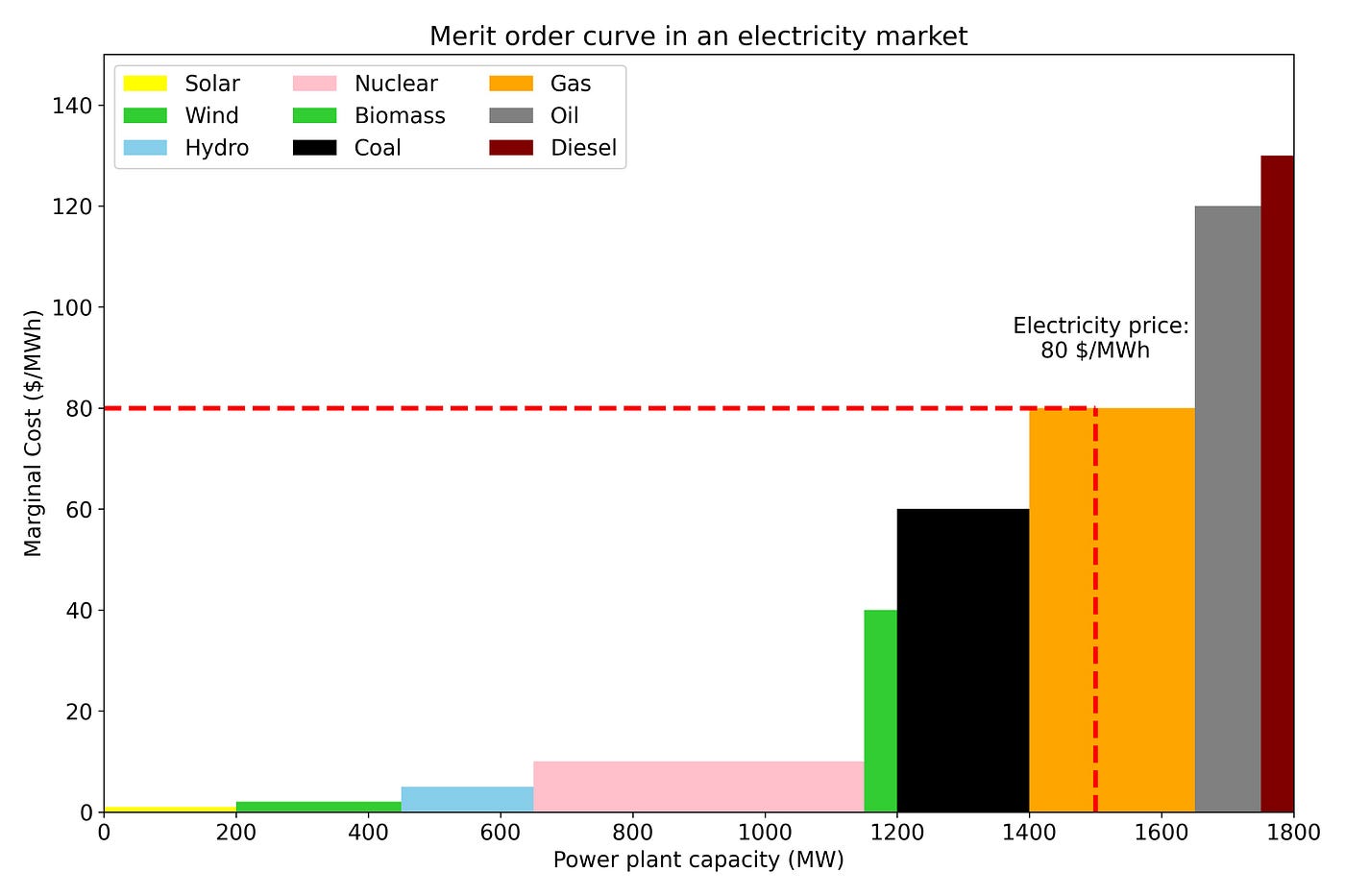
^{Merit orders electrical curve provided. Ix-axis represents the available capacity for energy plants. Iy-axis represents the right cost of each of the power plant. The red red line represents the need with gas. The horizontal red line represents the cost of electrical generation from electricity, which puts the price of cleaning market. Photo by author.}

In the outgoing gossip, the demand for 1500 MW is portrayed by a vertical red line. This is in line with the provision of energy from electricity where all energy plants are organized by climbing a side order. Therefore, the costs of the electrical generation from electricity IE 80 $ / MWH price of market. This means all energy plants before and before the red red-owned lines held in X-axis ee solar, air, nuclear, and gas requires to bring power to meet the need. And they all find the price set by the back cost of the production from the electricity.

Order Order Effect

When the demands of the demands change in energy system, the total electricity is also responsive. This is displayed in the GIF picture below. Getting photos of Python, I used interact work from ipywidgets as shown below. I also used IntSlider The widget to set updemand as a parameter described by a user of contact. To avoid fullness while dragging with slide, I have said continuous_update It's false.

from ipywidgets import *
demand = widgets.IntSlider(
                value = 100,
                min = 0,
                max = df[“Available capacity (MW)”].sum(),
                step = 10, 
                description = “Demand”,
                continuous_update = False #False to avoid flickering
                )
interactive_plot = interact(merit_order_curve, demand = demand)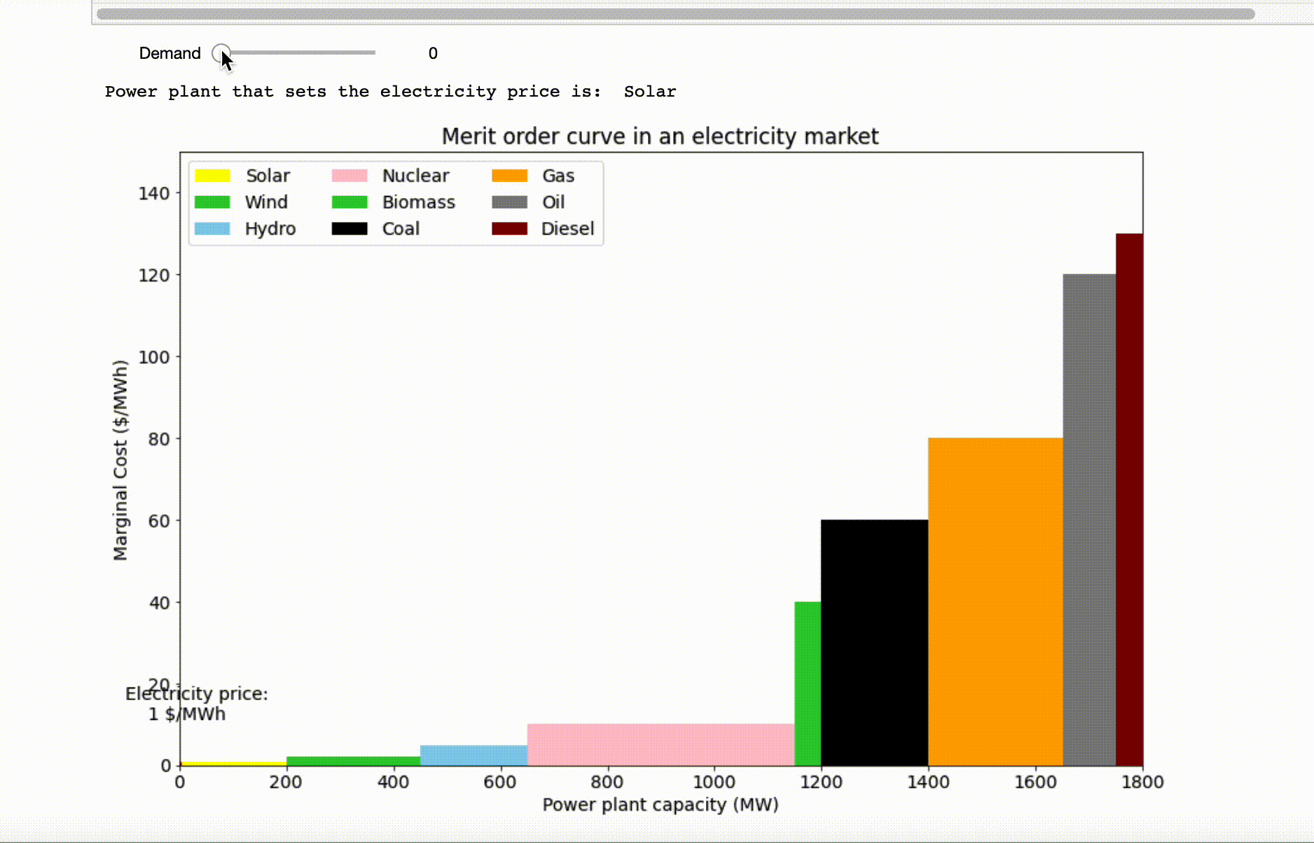

^{Animation indicates changes in reducing power plant and a perfect electric price such as change for need. Photo by author.}

As shown in GIF image above, when the need increases, many energy plants look at the right of the appropriate commandment they need to ship, suggesting the price of cleaning and contrary. If there is an extraordinary capacity of renewable energy plants in the portfolio, the further assignment is required by renewable resources. This often reduces the price of electricity, known as Order Order Effect.

The Marginal Adatement calls a curve

This page Final Cost It is carried by the removal companies or reduced external equipment (bad byproducts) created during production. Once Cost of Side-Side Cost It measures the cost of reducing one additional unit of external items, e.g. While the curve of the Merit is based on the order of the order at the expense of the production, Mask Atatements (Mac) depending on the increased costs of increased costs of the rising cost of the rear cost.

In Mac curve, Bar width represents Greenhouse Gas (GHG) reductions of any decrease in any technology or option. And the bar is the costs of reducing one additional unit of ghg issuing about a given opportunity.
^{The DataFrame contains potential costs and the final cost of the final sides of different opportunities. Data is based on the writer's thinking.}

Details of this example is based on my thinking and can be considered as dummy data. Mac Curve Curve Epython is similar to that of the Merit Order Curve.

^{Mac turns somebody else's year X. Photos are the author.}

Bar width represents the reduction of the GHG year to exit opportunities for reducing. The bar in the bar is to symbolize estimated costs in a year provided to reduce from 1 TCO2E.

As indicated in the above building, we return the old lights with light lamps is the most expensive way of the devartonn. Unfortunate costs for attacks after specific opportunities mean that there is money paid (or profits) when those measures are used. As we move on to the end of the X-axis to the Mac curve, it is very expensive to leave one unit of exits GHG. The largest bar in the mac curve, redesigning is the highest powers of the GHG output.

Therefore, the MAC curve allows steps from various fields (HERE POWER, transport, properties, forests, and waste) to compare with the same names. While the MAC turns provides basic assessment of the income and the operation of various mining costs, including the testing of other moderately provides a powerful basis for investing policies and investment decisions.

Store

As we pass through the global power, many fat swinging to meet the needs of our energy can lead to the sooner the outcome budget. There is also provincial and economic opportunities, can reduce the GHG out of both Energy and Nongy Energy Energy Energy. In addition, with the economy of the average, preliminary reduction technology (eg air and light) they are cheap every year.
It is important to use preliminary technology options to reduce the physical out of the body. Reduction options come from their cost and benefits. In this post, I discussed that the renewable power assignment and Fossil Feels in the portfolio of the country's power system influence the total electricity prices in the sense of the Merit Order Curve (Based on the Costside Cost of Manufacturing). And I introduce the decline in the improvement of results how can it work and works well with the cost of reducing the country's reduction expenses can be tested based on the The Marginal Adatement calls a curve. The implementation of these curves epython is found in this storage giver.