
Machines don’t break down out of nowhere—there are always signs. The problem? Humans aren’t always great at noticing them. That’s where Machine Predictive Maintenance comes in! This guide will take you through the exciting world of Machine Predictive Maintenance, using AWS and MLOps to ensure your equipment stays predictably reliable.
Learning Objectives
- Understand how to design and implement an end-to-end MLOps pipeline for predictive maintenance, covering data ingestion, model training, and deployment.
- Learn to integrate essential tools like Docker, FastAPI, and AWS services to build a robust, production-ready machine learning application.
- Explore the use of GitHub Actions for automating CI/CD workflows, ensuring smooth and reliable code integration and deployment.
- Set up best practices for monitoring, performance tracking, and continuous improvement to keep your machine learning models efficient and maintainable.
This article was published as a part of the Data Science Blogathon.
Problem: Unplanned Downtime & Maintenance Costs
Unexpected equipment failures in industrial settings cause downtime and financial losses. In our project, we are using MLOps best practices and machine learning to detect issues early, enabling timely repairs and reducing disruptions.
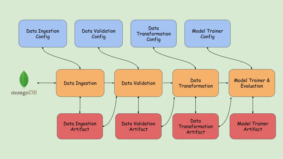
Before diving into implementation, let’s take a closer look at the project architecture.
Necessary Prerequisites
Below we will first look in the prerequisites required:
Clone the repository:
git clone "
cd Predictive_Maintenance_MLOps
Create and activate the virtual environment:
# For macOS and Linux:
python3 -m venv venv
source venv/bin/activate

# For Windows:
python -m venv venv
.venvScriptsactivate
Install Required Dependencies:
pip install -r requirements.txtSet Up Environment Variables:
# Create a `.env` file and add your MongoDB connection string:
MONGO_URI=your_mongodb_connection_string
Project Structure
The Project Structure outlines the key components and organization of the project, ensuring clarity and maintainability. It helps in understanding how different modules interact and how the overall system is designed. A well-defined structure simplifies development, debugging, and scalability.
project_root/
│
├── .github/
│   └── workflows/
│       └── main.yml
│
├── data_schema/
│   └── schema.yaml
│
├── final_model/
│   ├── model.pkl
│   └── preprocessor.pkl
│
├── Machine_Predictive_Data/
│   └── predictive_maintenance.csv
│
├── machine_predictive_maintenance/
│   ├── cloud/
│   ├── components/
│   ├── constant/
│   ├── entity/
│   ├── exception/
│   ├── logging/
│   ├── pipeline/
│   ├── utils/
│   └── __init__.py
│
├── my_venv/
│
├── notebooks/
│   ├── EDA.ipynb
│   ├── prediction_output/
│
├── templates/
│   └── table.html
│
├── valid_data/
|    └──test.csv
│
├── .env
├── .gitignore
├── app.py
├── Dockerfile
├── main.py
├── push_data.py
├── README.md
├── requirements.txt
├── setup.py
├── test_mongodb.py
Data Ingestion
In this project, we use a machine predictive maintenance CSV file, converting it into JSON records, and inserting it into a MongoDB collection.
Dataset Link:
Here is the code snippet to convert CSV -> JSON records -> MongoDB
class PredictiveDataExtract():

    def __init__(self):
        """
        Initializes the PredictiveDataExtract class.
        """
        try:
            pass
        except Exception as e:
            raise MachinePredictiveMaintenanceException(e, sys)

    def csv_to_json_convertor(self, file_path):
        try:
            data = pd.read_csv(file_path)
            data.reset_index(drop=True, inplace=True)
            records = list(json.loads(data.T.to_json()).values())
            return records
        except Exception as e:
            raise MachinePredictiveMaintenanceException(e, sys)

    def insert_data_mongodb(self, records, database, collection):
        try:
            self.records = records
            self.database = database
            self.collection = collection

            self.mongo_client = pymongo.MongoClient(MONGO_DB_URL)
            self.database = self.mongo_client[self.database]

            self.collection = self.database[self.collection]
            self.collection.insert_many(self.records)
            return(len(self.records))
        except Exception as e:
            raise MachinePredictiveMaintenanceException(e, sys)

if __name__=="__main__":
    FILE_PATH="Machine_Predictive_Data/predictive_maintenance.csv"
    DATABASE="Predictive_Maintenance_MLOps"
    collection = "Machine_Predictive_Data"

    predictive_data_obj=PredictiveDataExtract()
    records = predictive_data_obj.csv_to_json_convertor(FILE_PATH)
    no_of_records = predictive_data_obj.insert_data_mongodb(records, DATABASE, collection)
    print(no_of_records)
Here is the code snippet to fetch data from MongoDB, split the data into train and test CSV files, and store them as a Data Ingestion artifact.
class DataIngestion:
    def __init__(self, data_ingestion_config:DataIngestionConfig):

        """
        Initializes the DataIngestion class with the provided configuration.

        Parameters:
            data_ingestion_config: DataIngestionConfig
                Configuration object containing details for data ingestion.
        """
        try:
            self.data_ingestion_config=data_ingestion_config
        except Exception as e:
            raise MachinePredictiveMaintenanceException(e, sys)

    def export_collection_as_dataframe(self):
        try:
            database_name= self.data_ingestion_config.database_name
            collection_name= self.data_ingestion_config.collection_name
            self.mongo_client = pymongo.MongoClient(MONGO_DB_URL)
            collection = self.mongo_client[database_name][collection_name]
            df = pd.DataFrame(list(collection.find()))
            if "_id" in df.columns.to_list():
                df = df.drop(columns=["_id"], axis=1)
            df.replace({"na":np.nan},inplace=True)
            return df
        except Exception as e:
            raise MachinePredictiveMaintenanceException(e, sys)

    def export_data_into_feature_store(self,dataframe: pd.DataFrame):
        try:
            feature_store_file_path=self.data_ingestion_config.feature_store_file_path
            #creating folder
            dir_path = os.path.dirname(feature_store_file_path)
            os.makedirs(dir_path,exist_ok=True)
            dataframe.to_csv(feature_store_file_path,index=False,header=True)
            return dataframe
        except Exception as e:
            raise MachinePredictiveMaintenanceException(e,sys)

    def split_data_as_train_test(self, dataframe:pd.DataFrame):
        try:
            train_set, test_set = train_test_split(
                dataframe, test_size=self.data_ingestion_config.train_test_split_ratio
            )
            logging.info("Performed train test split on the dataframe")
            logging.info(
                "Exited split_data_as_train_test method of Data_Ingestion class"
            )
            dir_path = os.path.dirname(self.data_ingestion_config.training_file_path)
            os.makedirs(dir_path, exist_ok=True)
            logging.info(f"Exporting train and test file path.")
            train_set.to_csv(
                self.data_ingestion_config.training_file_path, index=False, header=True
            )
            test_set.to_csv(
                self.data_ingestion_config.testing_file_path, index=False, header=True
                            )
            logging.info(f"Exported train and test file path."  )
        except Exception as e:
            raise MachinePredictiveMaintenanceException(e, sys)

    def initiate_data_ingestion(self):
        try:
            dataframe = self.export_collection_as_dataframe()
            dataframe = self.export_data_into_feature_store(dataframe)
            self.split_data_as_train_test(dataframe)
            dataingestionartifact= DataIngestionArtifact(trained_file_path=self.data_ingestion_config.training_file_path,
                                                         test_file_path=self.data_ingestion_config.testing_file_path)
            return dataingestionartifact
        except Exception as e:
            raise MachinePredictiveMaintenanceException(e,sys)
Data Validation
In this step, we’ll check if the ingested data meets the expected format by ensuring all required columns are present using a predefined schema and comparing the training and testing data for any differences. Then we save the clean data and create a drift report, so only quality data is used for the next step, which is transforming the data.
Data Validation code snippet:
class DataValidation:

    def __init__(self, data_ingestion_artifact:DataIngestionArtifact,
                 data_validation_config: DataValidationConfig):
        try:
            self.data_ingestion_artifact= data_ingestion_artifact
            self.data_validation_config= data_validation_config
            self._schema_config = read_yaml_file(SCHEMA_FILE_PATH)
        except Exception as e:
            raise MachinePredictiveMaintenanceException(e, sys)

    @staticmethod
    def read_data(file_path) -> pd.DataFrame:
        try:
            return pd.read_csv(file_path)
        except Exception as e:
            raise MachinePredictiveMaintenanceException(e, sys)


    def validate_number_of_columns(self, dataframe:pd.DataFrame)-> bool:
        try:
            number_of_columns = len(self._schema_config)
            logging.info(f"Required number of columns:{number_of_columns}")
            logging.info(f"Data frame has columns:{len(dataframe.columns)}")

            if len(dataframe.columns) == number_of_columns:
                return True
            return False
        except Exception as e:
            raise MachinePredictiveMaintenanceException (e, sys)


    def is_columns_exist(self, df:pd.DataFrame) -> bool:
        try:
            dataframe_columns = df.columns
            missing_numerical_columns = []
            missing_categorical_columns = []

            for column in self._schema_config["numerical_columns"]:
                if column not in dataframe_columns:
                    missing_numerical_columns.append(column)

            if len(missing_numerical_columns) > 0:
                logging.info(f"Missing numerical column: {missing_numerical_columns}")

            for column in self._schema_config["categorical_columns"]:
                if column not in dataframe_columns:
                    missing_categorical_columns.append(column)

            if len(missing_categorical_columns) > 0:
                logging.info(f"Missing categorical column: {missing_categorical_columns}")
            return False if len(missing_categorical_columns)>0 or len(missing_numerical_columns)>0 else True

        except Exception as e:
            raise MachinePredictiveMaintenanceException(e, sys)


    def detect_dataset_drift(self, base_df, current_df, threshold = 0.05) -> bool :
        try:
            status = True
            report = {}
            for column in base_df.columns:
                d1 = base_df[column]
                d2 = current_df[column]

                is_same_dist = ks_2samp(d1, d2)
                if threshold <= is_same_dist.pvalue:
                    is_found = False

                else:
                    is_found = True
                    status = False

                report.update({column:{
                    "p_value": float(is_same_dist.pvalue),
                    "drift_status": is_found
                }})
            drift_report_file_path = self.data_validation_config.drift_report_file_path
            dir_path = os.path.dirname(drift_report_file_path)# create directory
            os.makedirs(dir_path, exist_ok=True)

            write_yaml_file(file_path=drift_report_file_path, content=report)
        except Exception as e:
            raise MachinePredictiveMaintenanceException(e, sys)

    def initiate_data_validation(self)-> DataValidationArtifact:
        try:
            validation_error_msg  = ""
            logging.info("Starting data validation")

            train_file_path = self.data_ingestion_artifact.trained_file_path
            test_file_path = self.data_ingestion_artifact.test_file_path

            # read the data from the train and test
            train_dataframe = DataValidation.read_data(train_file_path)
            test_dataframe = DataValidation.read_data(test_file_path)

            # validate number of columns
            status = self.validate_number_of_columns(dataframe=train_dataframe)
            logging.info(f"All required columns present in training dataframe: {status}")

            if not status:
                validation_error_msg += f"Train dataframe does not contain all columns.n"

            status = self.validate_number_of_columns(dataframe=test_dataframe)

            if not status:
                validation_error_msg += f"Test dataframe does not contain all columns.n"

            status = self.is_columns_exist(df=train_dataframe)

            if not status:
                validation_error_msg += f"Columns are missing in training dataframe."

            status = self.is_columns_exist(df=test_dataframe)

            if not status:
                validation_error_msg += f"columns are missing in test dataframe."
            ## lets check datadrift
            status=self.detect_dataset_drift(base_df=train_dataframe,current_df=test_dataframe)
            dir_path=os.path.dirname(self.data_validation_config.valid_train_file_path)
            os.makedirs(dir_path,exist_ok=True)

            train_dataframe.to_csv(
                self.data_validation_config.valid_train_file_path, index=False, header=True

            )
            test_dataframe.to_csv(
                self.data_validation_config.valid_test_file_path, index=False, header=True
            )

            data_validation_artifact = DataValidationArtifact(
                validation_status=status,
                valid_train_file_path=self.data_validation_config.valid_train_file_path,
                valid_test_file_path=self.data_validation_config.valid_test_file_path,
                invalid_train_file_path=None,
                invalid_test_file_path=None,
                drift_report_file_path=self.data_validation_config.drift_report_file_path,
            )
            return data_validation_artifact
        except Exception as e:
            raise MachinePredictiveMaintenanceException(e,sys)
Below is the drift report generated by the Data Validation.
Air temperature [K]:
  drift_status: true
  p_value: 0.016622943467175914
Failure Type:
  drift_status: false
  p_value: 1.0
Process temperature [K]:
  drift_status: false
  p_value: 0.052940072765804994
Product ID:
  drift_status: false
  p_value: 0.09120557172716418
Rotational speed [rpm]:
  drift_status: false
  p_value: 0.2673520066245566
Target:
  drift_status: false
  p_value: 0.999999998717466
Tool wear [min]:
  drift_status: false
  p_value: 0.13090856779628832
Torque [Nm]:
  drift_status: false
  p_value: 0.5001773464540389
Type:
  drift_status: false
  p_value: 1.0
UDI:
  drift_status: true
  p_value: 0.022542489133976953
Data Transformation
Here, we will clean and transform the validated data by converting temperature features from Kelvin to Celsius, dropping unnecessary columns, and applying a transformation pipeline that uses ordinal encoding and Min-Max scaling, and handling data imbalance using SMOTEENN.
The transformed training and test datasets are saved as .npy files along with a serialized preprocessing object i.e. Minmax scaler(preprocessing.pkl) all encapsulated as an artifact for further model training.
class DataTransformation:

    def __init__(self,data_validation_artifact: DataValidationArtifact,
                 data_transformation_config: DataTransformationConfig):
        try:
            self.data_validation_artifact: DataValidationArtifact = data_validation_artifact
            self.data_transformation_config: DataTransformationConfig = data_transformation_config
            self._schema_config = read_yaml_file(file_path=SCHEMA_FILE_PATH)
        except Exception as e:
            raise MachinePredictiveMaintenanceException(e,sys)

    @staticmethod
    def read_data(file_path) -> pd.DataFrame:
        try:
            return pd.read_csv(file_path)
        except Exception as e:
            raise MachinePredictiveMaintenanceException(e, sys)

    def get_data_transformer_object(self):
        try:
            logging.info("Got numerical cols from schema config")

            scaler = MinMaxScaler()
            # Fetching categories for OrdinalEncoder from schema config
            ordinal_categories = self._schema_config.get('ordinal_categories', [])
            ordinal_encoder = OrdinalEncoder(categories=ordinal_categories)

            logging.info("Initialized MinMaxScaler, OrdinalEncoder with categories")

            ordinal_columns = self._schema_config['ordinal_columns']
            scaling_features = self._schema_config['scaling_features']
            preprocessor = ColumnTransformer(
                [
                    ("Ordinal_Encoder", ordinal_encoder, ordinal_columns),
                    ("MinMaxScaling", scaler, scaling_features)
                ]
            )
            logging.info("Created preprocessor object from ColumnTransformer")
            return preprocessor
        except Exception as e:
            raise MachinePredictiveMaintenanceException(e, sys)

    def initiate_data_transformation(self) -> DataTransformationArtifact:
        try:

            logging.info("Starting data transformation")
            preprocessor = self.get_data_transformer_object()
            train_df = DataTransformation.read_data(self.data_validation_artifact.valid_train_file_path)
            test_df = DataTransformation.read_data(self.data_validation_artifact.valid_test_file_path)
            input_feature_train_df = train_df.drop(columns=[TARGET_COLUMN], axis=1)
            target_feature_train_df = train_df[TARGET_COLUMN]

            input_feature_train_df['Air temperature [c]'] = input_feature_train_df['Air temperature [K]'] - 273.15
            input_feature_train_df['Process temperature [c]'] = input_feature_train_df['Process temperature [K]'] - 273.15
            drop_cols = self._schema_config['drop_columns']

            input_feature_train_df = drop_columns(df=input_feature_train_df, cols = drop_cols)
            logging.info("Completed dropping the columns for Training dataset")
            input_feature_test_df = test_df.drop(columns=[TARGET_COLUMN], axis=1)
            target_feature_test_df = test_df[TARGET_COLUMN]

            input_feature_test_df['Air temperature [c]'] = input_feature_test_df['Air temperature [K]'] - 273.15
            input_feature_test_df['Process temperature [c]'] = input_feature_test_df['Process temperature [K]'] - 273.15
            drop_cols = self._schema_config['drop_columns']
            input_feature_test_df = drop_columns(df=input_feature_test_df, cols = drop_cols)

            logging.info("Completed dropping the columns for Testing dataset")
            input_feature_train_arr = preprocessor.fit_transform(input_feature_train_df)
            input_feature_test_arr = preprocessor.transform(input_feature_test_df)

            smt =  SMOTEENN(sampling_strategy="minority")
            input_feature_train_final, target_feature_train_final = smt.fit_resample(
                input_feature_train_arr, target_feature_train_df
            )
            logging.info("Applied SMOTEENN on training dataset")

            input_feature_test_final, target_feature_test_final = smt.fit_resample(
                input_feature_test_arr, target_feature_test_df
            )
            train_arr = np.c_[
                input_feature_train_final, np.array(target_feature_train_final)
            ]
            test_arr = np.c_[
                input_feature_test_final, np.array(target_feature_test_final)
            ]
            save_numpy_array_data(self.data_transformation_config.transformed_train_file_path, array=train_arr, )
            save_numpy_array_data(self.data_transformation_config.transformed_test_file_path,array=test_arr,)
            save_object( self.data_transformation_config.transformed_object_file_path, preprocessor,)

            save_object( "final_model/preprocessor.pkl", preprocessor,)

            data_transformation_artifact=DataTransformationArtifact(
                transformed_object_file_path=self.data_transformation_config.transformed_object_file_path,
                transformed_train_file_path=self.data_transformation_config.transformed_train_file_path,
                transformed_test_file_path=self.data_transformation_config.transformed_test_file_path
            )
            return data_transformation_artifact
        except Exception as e:
            raise MachinePredictiveMaintenanceException(e, sys)
Training and Evaluation
Now we will train different classification models on the transformed training data like Decision Tree, Random Forest, Gradient Boosting, Logistic Regression, and AdaBoost models and evaluate their performance using evaluation metrics like f1-score, precision, and recall, and then log these details with MLflow.
After selecting the best model, it saves both the model and transformation object locally to artifact and evaluation metrics to use it for deployment.
class ModelTrainer:
    def __init__(self, data_transformation_artifact: DataTransformationArtifact, model_trainer_config: ModelTrainerConfig):
        try:
            self.data_transformation_artifact = data_transformation_artifact
            self.model_trainer_config = model_trainer_config

        except Exception as e:
            raise MachinePredictiveMaintenanceException(e, sys)

    def track_mlflow(self, best_model, classification_metric, input_example):
        """
        Log model and metrics to MLflow.

        Args:
            best_model: The trained model object.
            classification_metric: The classification metrics (f1, precision, recall).
            input_example: An example input data sample for the model.
        """
        try:
            with mlflow.start_run():
                f1_score=classification_metric.f1_score
                precision_score=classification_metric.precision_score
                recall_score=classification_metric.recall_score

                mlflow.log_metric("f1_score",f1_score)
                mlflow.log_metric("precision",precision_score)
                mlflow.log_metric("recall_score",recall_score)
                mlflow.sklearn.log_model(best_model,"model", input_example=input_example)
        except Exception as e:
            raise MachinePredictiveMaintenanceException(e, sys)

    def train_model(self, X_train, y_train, X_test, y_test ):
        """
        Train multiple models and select the best-performing one based on evaluation metrics.

        Args:
            X_train: Training features.
            y_train: Training labels.
            X_test: Testing features.
            y_test: Testing labels.

        Returns:
            ModelTrainerArtifact: An artifact containing details about the trained model and its metrics.
        """
        models = {
                "Random Forest": RandomForestClassifier(verbose=1),
                "Decision Tree": DecisionTreeClassifier(),
                "Gradient Boosting": GradientBoostingClassifier(verbose=1),
                "Logistic Regression": LogisticRegression(verbose=1),
                "AdaBoost": AdaBoostClassifier(),
            }
        params={
            "Decision Tree": {
                'criterion':['gini', 'entropy', 'log_loss'],
                # 'splitter':['best','random'],
                # 'max_features':['sqrt','log2'],
            },
            "Random Forest":{
                # 'criterion':['gini', 'entropy', 'log_loss'],

                # 'max_features':['sqrt','log2',None],
                'n_estimators': [8,16,32,128,256]
            },
            "Gradient Boosting":{
                # 'loss':['log_loss', 'exponential'],
                'learning_rate':[.1,.01,.05,.001],
                'subsample':[0.6,0.7,0.75,0.85,0.9],
                # 'criterion':['squared_error', 'friedman_mse'],
                # 'max_features':['auto','sqrt','log2'],
                'n_estimators': [8,16,32,64,128,256]
            },
            "Logistic Regression":{},
            "AdaBoost":{
                'learning_rate':[.1,.01,.001],
                'n_estimators': [8,16,32,64,128,256]
            }

        }
        model_report: dict = evaluate_models(X_train=X_train, y_train=y_train, X_test=X_test, y_test=y_test,
                                             models=models, param=params)
        best_model_score = max(sorted(model_report.values()))
        logging.info(f"Best Model Score: {best_model_score}")
        best_model_name = list(model_report.keys())[
            list(model_report.values()).index(best_model_score)
        ]
        logging.info(f"Best Model Name: {best_model_name}")
        best_model = models[best_model_name]

        y_train_pred = best_model.predict(X_train)
        classification_train_metric = get_classification_score(y_true=y_train, y_pred=y_train_pred)

        input_example = X_train[:1]
        print(input_example)
        # Track the experiments with mlflow
        self.track_mlflow(best_model, classification_train_metric, input_example)


        y_test_pred=best_model.predict(X_test)
        classification_test_metric = get_classification_score(y_true=y_test, y_pred=y_test_pred)

        # Track the experiments with mlflow
        self.track_mlflow(best_model, classification_test_metric, input_example)


        preprocessor = load_object(file_path=self.data_transformation_artifact.transformed_object_file_path)


        model_dir_path = os.path.dirname(self.model_trainer_config.trained_model_file_path)
        os.makedirs(model_dir_path,exist_ok=True)

        Machine_Predictive_Model = MachinePredictiveModel(model=best_model)

        save_object(self.model_trainer_config.trained_model_file_path,obj=MachinePredictiveModel)

        save_object("final_model/model.pkl",best_model)

        ## Model Trainer Artifact
        model_trainer_artifact=ModelTrainerArtifact(trained_model_file_path=self.model_trainer_config.trained_model_file_path,
                             train_metric_artifact=classification_train_metric,
                             test_metric_artifact=classification_test_metric
                             )
        logging.info(f"Model trainer artifact: {model_trainer_artifact}")
        return model_trainer_artifact

    def initiate_model_trainer(self) -> ModelTrainerArtifact:

        try:
            train_file_path = self.data_transformation_artifact.transformed_train_file_path
            test_file_path = self.data_transformation_artifact.transformed_test_file_path

            #loading training array and testing array
            train_arr = load_numpy_array_data(train_file_path)
            test_arr = load_numpy_array_data(test_file_path)

            X_train, y_train, X_test, y_test = (
                train_arr[:, :-1],
                train_arr[:, -1],
                test_arr[:, :-1],
                test_arr[:, -1],
            )

            model_trainer_artifact=self.train_model(X_train,y_train,X_test,y_test)
            return model_trainer_artifact

        except Exception as e:
            raise MachinePredictiveMaintenanceException(e, sys)
Now, let’s create a training_pipeline.py file where we sequentially integrate all the steps of data ingestion, validation, transformation, and model training into a complete pipeline.
def run_pipeline(self):

        """
        Executes the entire training pipeline.

        Returns:
            ModelTrainerArtifact: Contains metadata about the trained model.
        """
        try:
            data_ingestion_artifact= self.data_ingestion()
            data_validation_artifact= self.data_validation(data_ingestion_artifact=data_ingestion_artifact)
            data_transformation_artifact= self.data_transformation(data_validation_artifact=data_validation_artifact)
            model_trainer_artifact= self.model_trainer(data_transformation_artifact=data_transformation_artifact)
            self.sync_artifact_dir_to_s3()
            self.sync_saved_model_dir_to_s3()

            return model_trainer_artifact
        except Exception as e:
            raise MachinePredictiveMaintenanceException(e,sys)
You can visually see how we have built the training_pipeline.
Now that we’ve completed creating the pipeline, run the training_pipeline.py file to view the artifacts generated in the previous steps.
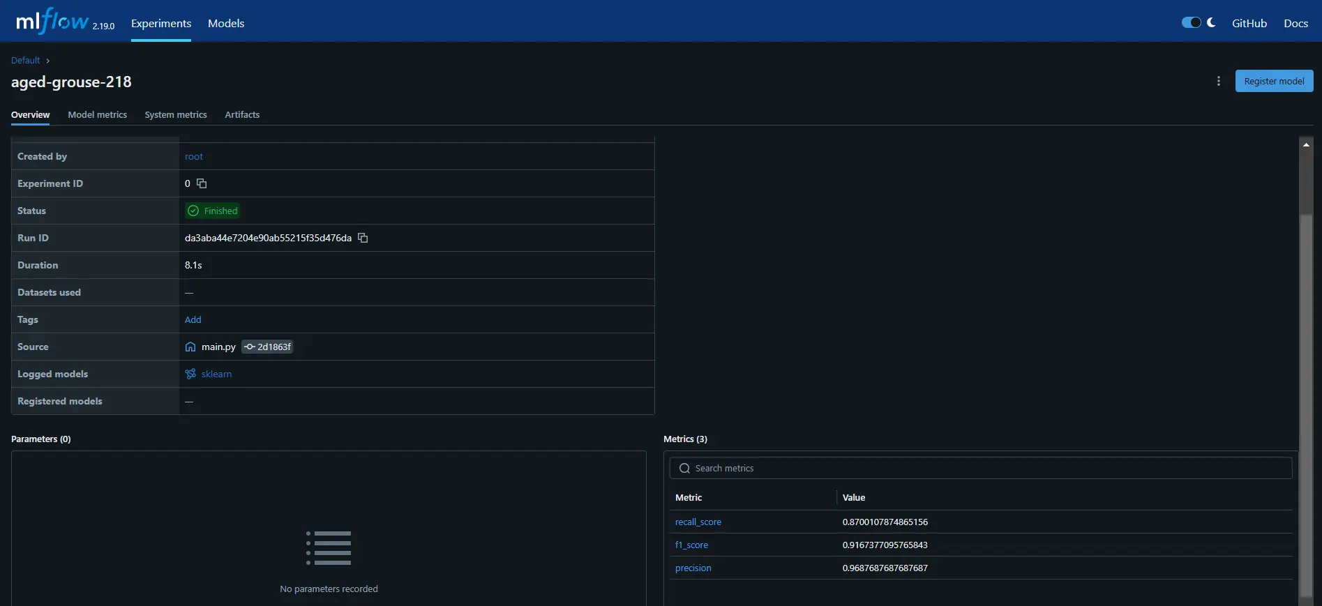
python training_pipeline.pyRun the following command to view the MLflow dashboard.
mlflow ui # Launch the MLflow dashboard to monitor experiments.As you can see, we have successfully logged model metrics like recall, precision, and F1-score in MLflow.
AWS Integration
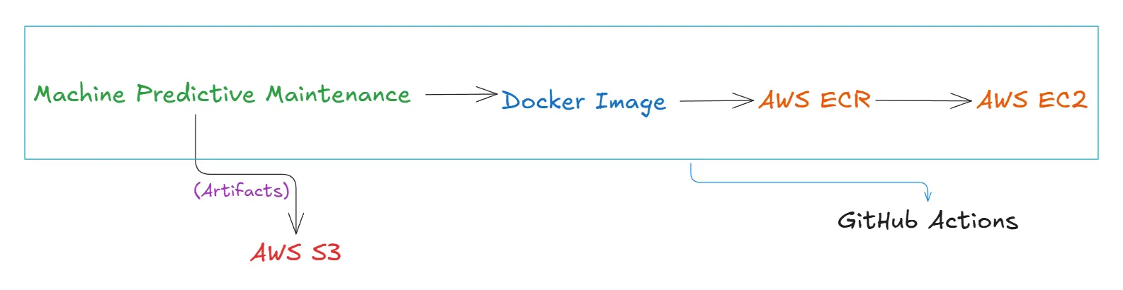
After running the training_pipeline.py file, we generated artifacts and stored them locally. Now, we will store these artifacts in an AWS S3 bucket to enable cloud-based storage and accessibility.
Using a Docker image, we will push it to AWS ECR via GitHub Actions and then deploy it to production using AWS EC2. We will discuss this process in more detail in the upcoming sections.
AWS S3
Follow these steps to create an AWS S3 bucket:
Step1: Download AWS CLI
- You can click here to download AWS CLI for Windows, Linux, and macOS
Step2: Log in to AWS IAM User
- You can sign in to the Console with your IAM user credentials and select the appropriate AWS region (eg., us-east-1).
- Once logged in, search for ‘IAM’ in the AWS search bar. Navigate to ‘Users,’ select your username, and go to the ‘Security Credentials’ tab. Under ‘Access Keys,’ click ‘Create access key,’ choose ‘CLI,’ and then confirm by clicking ‘Create access key’.
- Now, open your terminal and type aws configure. Enter your AWS Access Key and Secret Access Key when prompted, then press Enter.
Your IAM user has been successfully connected to your project.
Step3: Navigate to S3 Service
- Once logged in, search for “S3” in the AWS search bar.
- Click on Amazon S3 service and select the “Create bucket” button. Next, type in a unique bucket name (eg., machinepredictive)
- Review the configuration settings, and then click on “Create bucket.”
Your bucket is now created, and you can start uploading artifacts. Now, add the following code to your training_pipeline.py file and run it again to see the artifacts in your AWS S3 bucket.
    def sync_artifact_dir_to_s3(self):

        """
        Syncs the artifact directory to S3.
        """
        try:

            aws_bucket_url = f"s3://{TRAINING_BUCKET_NAME}/artifact/{self.training_pipeline_config.timestamp}"
            self.s3_sync.sync_folder_to_s3(folder = self.training_pipeline_config.artifact_dir,aws_bucket_url=aws_bucket_url)

        except Exception as e:
            raise MachinePredictiveMaintenanceException(e,sys)

    def sync_saved_model_dir_to_s3(self):

        """
        Syncs the saved model directory to S3.
        """

        try:
            aws_bucket_url = f"s3://{TRAINING_BUCKET_NAME}/final_model/{self.training_pipeline_config.timestamp}"
            self.s3_sync.sync_folder_to_s3(folder = self.training_pipeline_config.model_dir,aws_bucket_url=aws_bucket_url)
        except Exception as e:
            raise MachinePredictiveMaintenanceException(e,sys)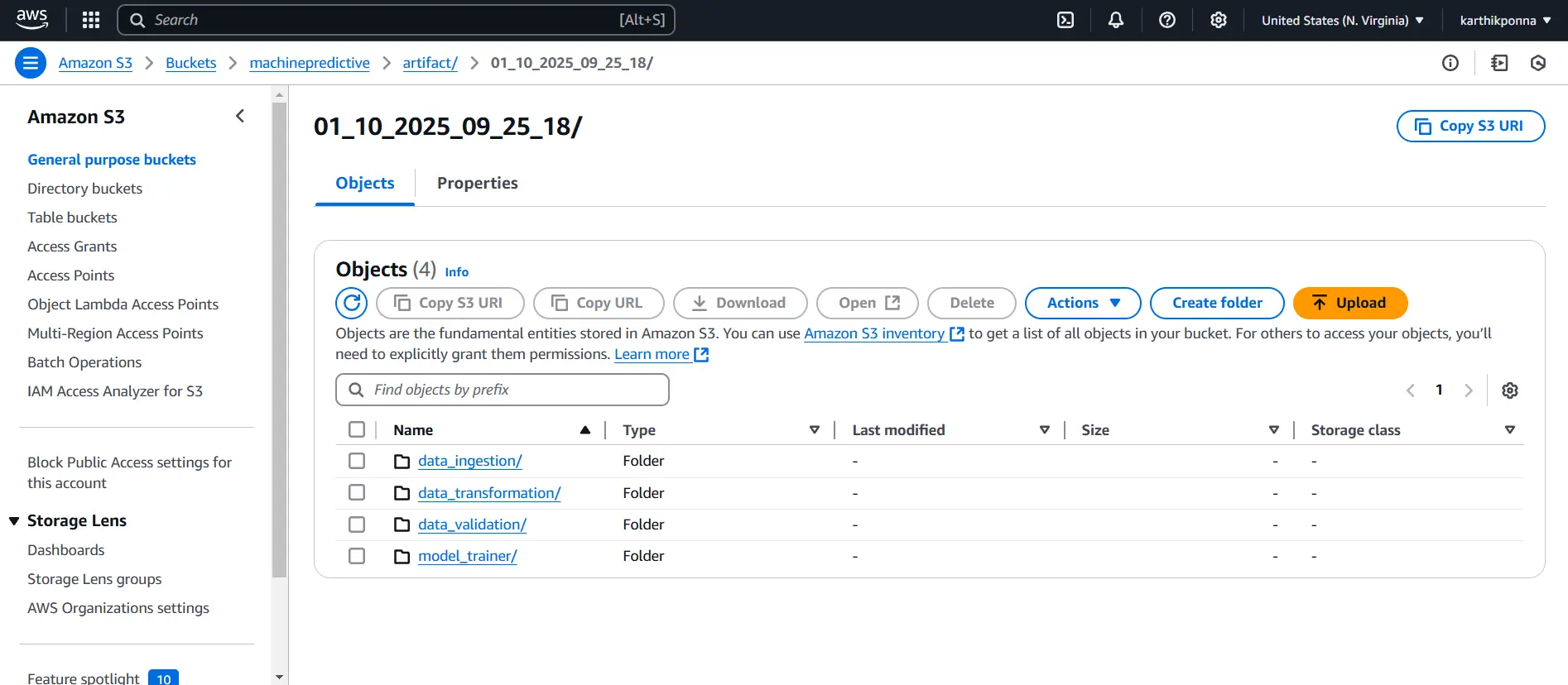
Amazon Elastic Container Registry (ECR)
Follow these steps to create an ECR repository.
- Search for ‘ECR’ in the AWS search bar.
- Click Create Repository, and select Private Repository.
- Provide a repository name (e.g., machinepredictive) and click Create.
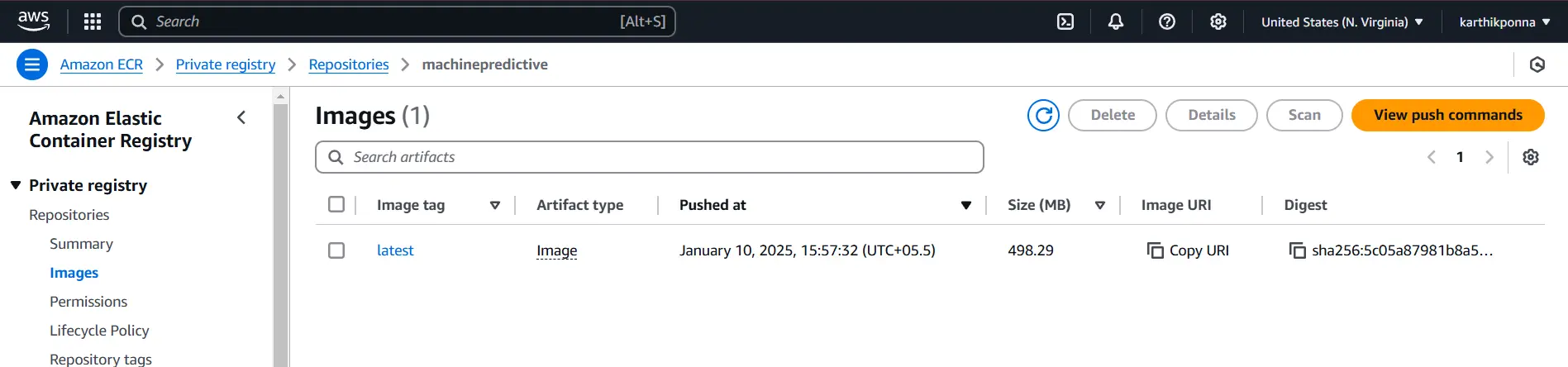
Copy the URI from your ECR repository, which should look something like “788614365622.dkr.ecr.ap-southeast-2.amazonaws.com“, and save it somewhere. We will need it later to paste into GitHub Secrets.
Docker Integration for Deployment
Dockerizing our project ensures it runs smoothly in any environment without dependency issues. It’s a must-have tool for packaging and sharing applications effortlessly.
Keeping the Docker image as small as possible is important for efficiency. We can minimize its size by using techniques like multi-staging and choosing a lightweight Python base image.
FROM python:3.10-slim-buster
WORKDIR /app
COPY . /app

RUN apt update -y && apt install awscli -y

RUN apt-get update && pip install -r requirements.txt
CMD ["python3", "app.py"]
Setup Action Secrets and Variables
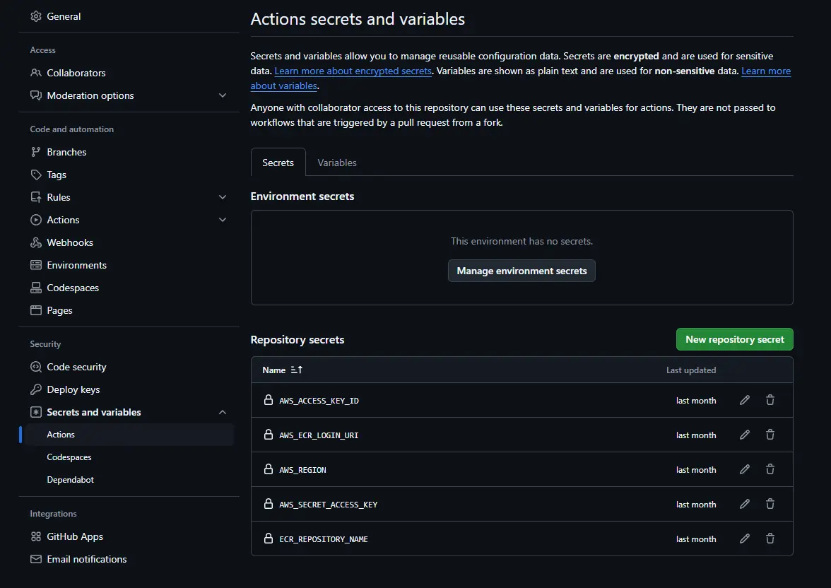
To securely store sensitive information like AWS credentials and repository URIs, we need to set up GitHub Action Secrets in our repository. Follow these steps:
Step1: Open Your GitHub Repository
Navigate to your repository on GitHub.
Step2: Go to Settings
At the top of your repository page, locate and click on the “Settings” tab.
Step3: Access Secrets and Variables
In the left sidebar, scroll down to Secrets and Variables → Select Actions.
Step4: Create a New Secret
Click the New repository secret button.
Step5: Add AWS Credentials
- Create a secret with the name “AWS_ACCESS_KEY_ID” and paste your AWS Access Key.
- Create another secret named AWS_SECRET_ACCESS_KEY and paste your AWS Secret Access Key.
- create a secret named “AWS_REGION” and paste your selected region (eg., us-east-1).
Step6: Add AWS ECR Repository URI
- Copy your ECR repository URI (e.g., 788614365622.dkr.ecr.ap-southeast-2.amazonaws.com).
- Create a new secret named “AWS_ECR_LOGIN_URI” and paste the copied URI.
- Create a new secret named “ECR_REPOSITORY_NAME” and paste the name of the ECR repository e.g., machinepredictive).
AWS EC2
Now let’s understand how to create an instance with AWS EC2. Follow these steps.
- Navigate to the EC2 service in the AWS Management Console and click Launch an instance.
- Name your instance (e.g., machinepredictive) and select Ubuntu as your operating system.
- Choose the instance type as t2.large.
- Select your default key pair.
- Under network security, choose the default VPC and configure the security groups as needed.
- Finally, click Launch Instance.
AWS EC2 CLI
After creating the instance named machinepredictive, select its Instance ID and click Connect. Then, under EC2 Instance Connect, click Connect again. This will open an AWS CLI interface where you can run the necessary commands.
Now, enter these commands in the CLI one by one to set up Docker on your EC2 instance:
sudo apt-get update -y
sudo apt-get upgrade
curl -fsSL -o get-docker.sh
sudo sh get-docker.sh
sudo usermod -aG docker ubuntu
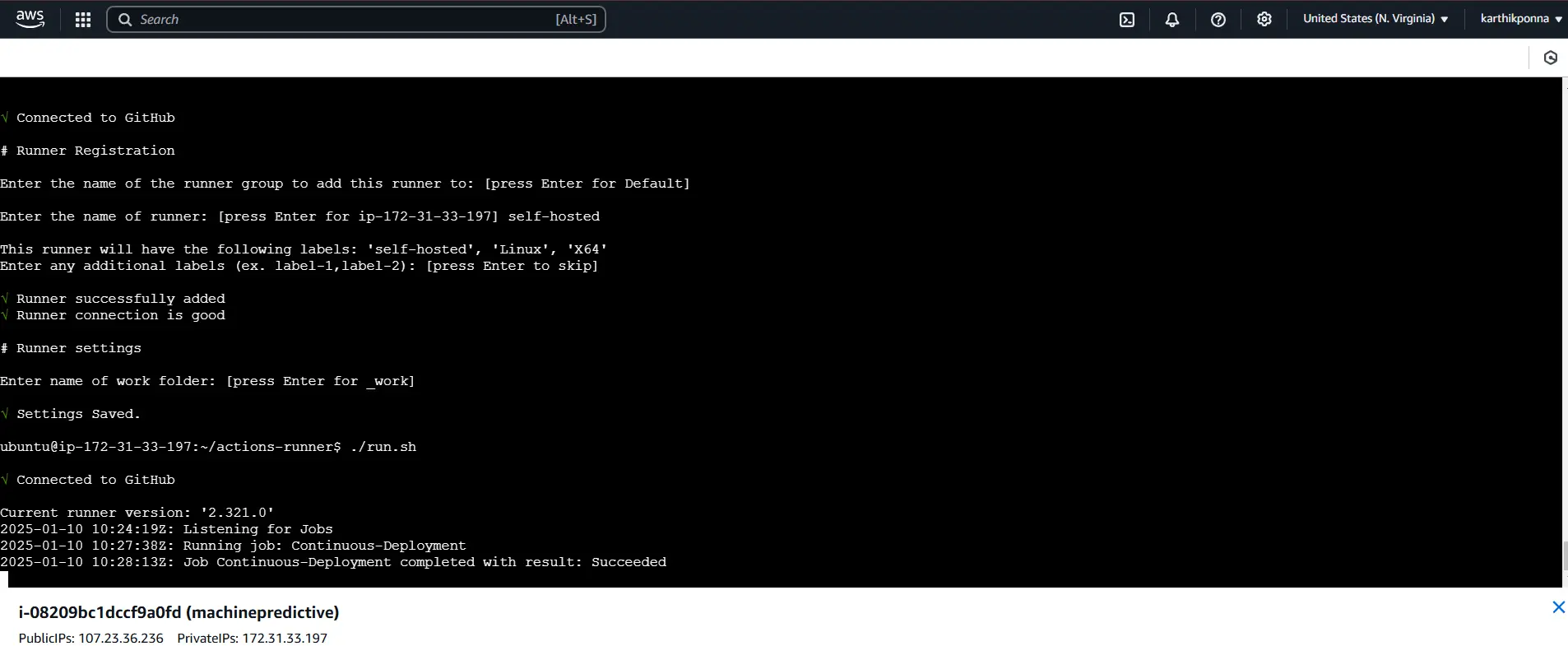
newgrp dockerKeep your CLI session open. Next, navigate to your GitHub repository, click on Settings, then go to the Actions section, and under Runners, click New self-hosted runner. Choose the Linux runner image. Now, run the following commands one by one in your CLI to download and configure your self-hosted runner:
# Create a folder and navigate into it
mkdir actions-runner && cd actions-runner

# Download the latest runner package
curl -o actions-runner-linux-x64-2.322.0.tar.gz -L

# Optional: Validate the hash
echo "b13b784808359f31bc79b08a191f5f83757852957dd8fe3dbfcc38202ccf5768  actions-runner-linux-x64-2.322.0.tar.gz" | shasum -a 256 -c

# Extract the installer
tar xzf ./actions-runner-linux-x64-2.322.0.tar.gz

# Configure the runner
./config.sh --url  --token "Paste your token here"

# Run the runner
./run.sh
This will download, configure, and start your self-hosted GitHub Actions runner on your EC2 instance.
After setting up the self-hosted GitHub Actions runner, the CLI will prompt you to enter a name for the runner. Type self-hosted and press Enter.
CI/CD with GitHub Actions
You can check out the .github/workflows/main.yml code file.
Now, let’s dive into what each section of this main.yml file does.
- Continuous Integration Job: This job runs on an Ubuntu runner to check out the code, lint it, and execute unit tests.
- Continuous Delivery Job: Triggered after CI, this job installs utilities, configures AWS credentials, logs into Amazon ECR, and builds, tags, and pushes your Docker image to ECR.
- Continuous Deployment Job: Running on a self-hosted runner, this job pulls the latest Docker image from ECR, runs it as a container to serve users, and cleans up any previous images or containers.
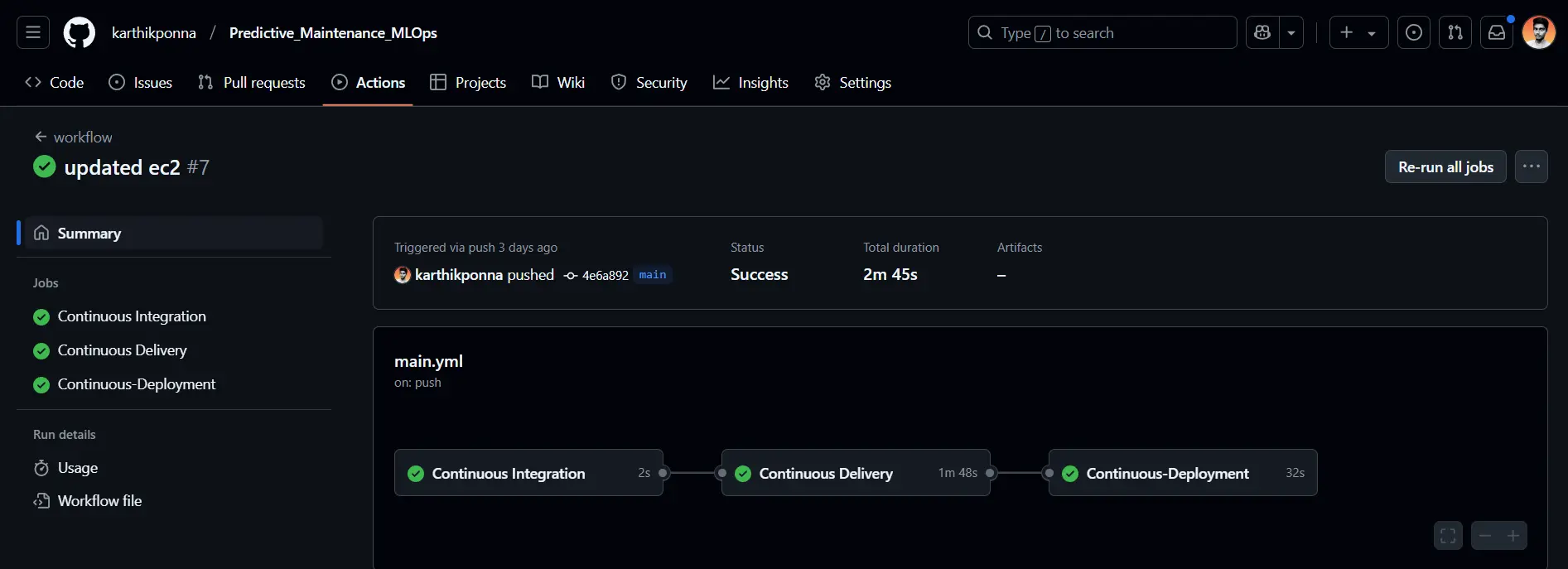
Once the Continuous Deployment Job completes successfully, you’ll see an output like this in the AWS CLI.
Open your AWS EC2 instance by clicking its Instance ID. Verify that the instance state is Running and locate the Public IPv4 DNS. Click on the “Open address” option to automatically launch your FastAPI application in your browser. Now, let’s dive into FastAPI.
FastAPI
You can check out the app.py file.
In this FastAPI application, I’ve created two main routes, one for training the model and another for generating predictions. Let’s explore each route in detail.
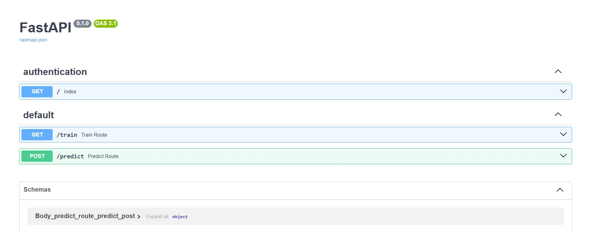
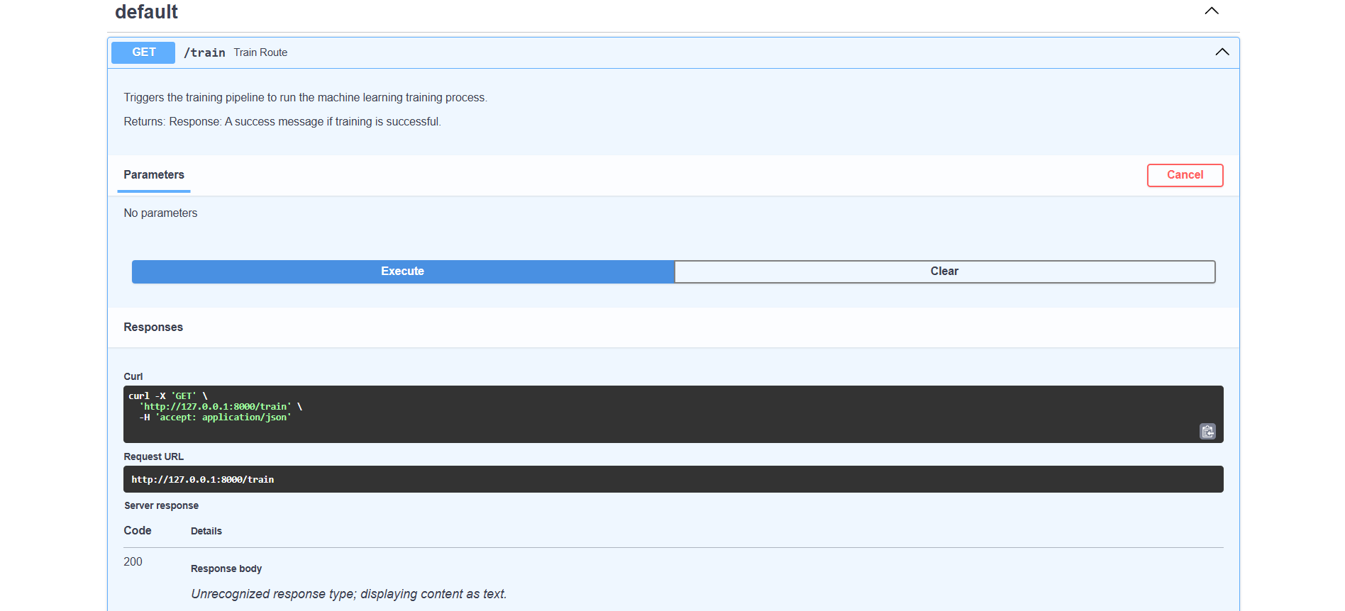
Train route
The /train endpoint starts the model training process using a predefined dataset, making it easy to update and improve the model with new data. It is especially useful for retraining the model to improve accuracy or incorporate new data, ensuring the model remains up-to-date and performs optimally.
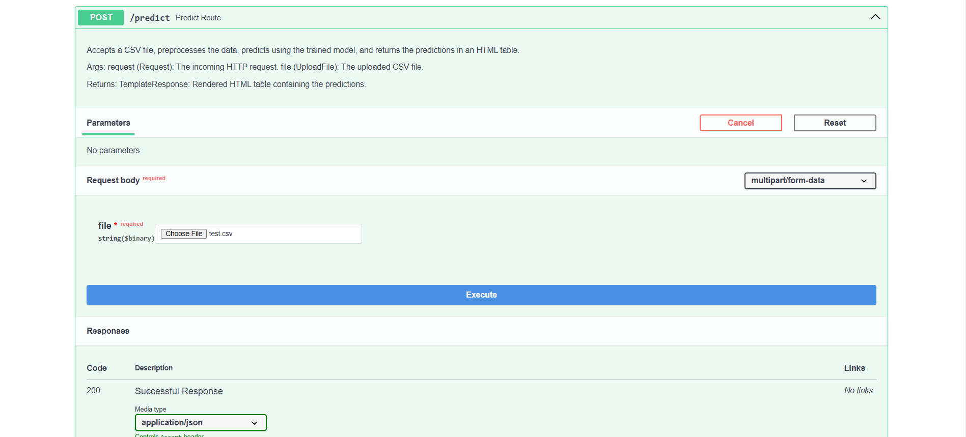
Predict route
The /predict endpoint accepts a CSV file via POST. This endpoint handles incoming data, leverages the trained model to generate predictions, and then returns the outcomes formatted as JSON. This route is perfect for applying the model to new datasets, making it efficient for large-scale prediction tasks.
In the /predict route, we’ve included a sample test.csv file; you can download it here.
Conclusion
Together, we built a full production-ready Predictive Maintenance MLOps project—from gathering and preprocessing data to training, evaluating, and deploying our model using Docker, AWS, and FastAPI. This project shows how MLOps can bridge the gap between development and production, making it easier to build robust, scalable solutions.
Remember, this guide is all about learning and applying these techniques to your data science projects. Don’t hesitate to experiment, innovate, and explore new enhancements as you progress. Thank you for sticking with me until the end—keep learning, keep doing, and keep growing!
GitHub repo:
Key Takeaways
- We built an end-to-end MLOps pipeline that covers data ingestion, model training, and deployment.
- Docker, AWS, and FastAPI work together seamlessly to move from development to production.
- Dockerizing our ML project is key—it ensures it runs smoothly in any environment without any dependency headaches.
- Continuous deployment ensures the model stays efficient and up-to-date in real-world applications.
Frequently Asked Questions
A. Docker ensures our ML project runs smoothly in any environment by eliminating dependency issues.
A. AWS services like EC2, S3, and ECR enable seamless deployment, storage, and scaling of our application.
A. MLflow makes machine learning development easier by offering tools for tracking experiments, versioning models, and deploying them.
A. GitHub Actions automates the CI/CD process—running tests, building Docker images, and deploying updates—ensuring a smooth transition from development to production.
The media shown in this article is not owned by Analytics Vidhya and is used at the Author’s discretion.
![]()
Hi! I’m Karthik Ponna, a Machine Learning Engineer at Antern. I’m deeply passionate about exploring the fields of AI and Data Science, as they constantly evolve and shape the future. I believe writing blogs is a great way to not only enhance my skills and solidify my understanding but also to share my knowledge and insights with others in the community. This helps me connect with like-minded individuals who share a curiosity for technology and innovation.


